|
|

Computed Tomography Image Quality
Optimization
and Dose Management
Perry Sprawls, Ph.D.
To step through module, CLICK
HERE.
To go to a specific topic
click on it below.
|
|
Computed Tomography Image Quality
Optimization
and Dose Management
Perry Sprawls, Ph.D.
To step through module, CLICK
HERE.
To go to a specific topic
click on it below.
|
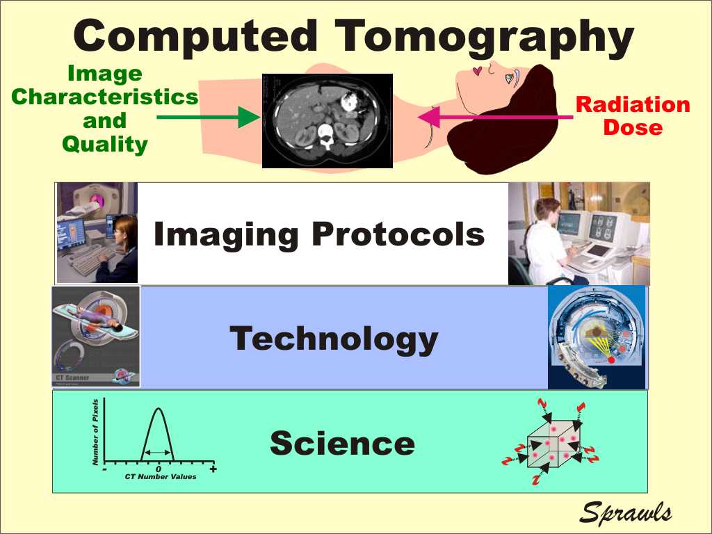
Computed tomography (CT) has the capability to provide
high-quality images for diagnostic procedures and visualization to guide
therapeutic procedures. It also imparts a relatively high
(compared to radiography) radiation dose to the patient's body.
Both the image quality characteristics
and the radiation
dose depend on and are controlled by the specific imaging protocol
selected for each patient. The protocol is made up of a complex
combination of many adjustable imaging factors or parameters for each
procedure. The objective for each imaging procedure is to adjust
the image characteristics to provide the required visualization of
anatomical structures and signs of pathology and limit the radiation
dose to no more than that required to produce the necessary image
quality. An underlying principle of all x-ray imaging, and especially CT, is that we "pay for" image quality with radiation dose. An optimized imaging protocol is one in which the factors are adjusted to provide the necessary image quality and visualization balanced against the radiation dose. In CT this is especially challenging because of the different image characteristics that must be considered and the rather complex way the radiation energy is distributed in the patient's body during a scan. In this module we will explore all of these factors and develop an understanding that help in developing and using optimized imaging protocols. It is all about how the scanner is operated! |
|
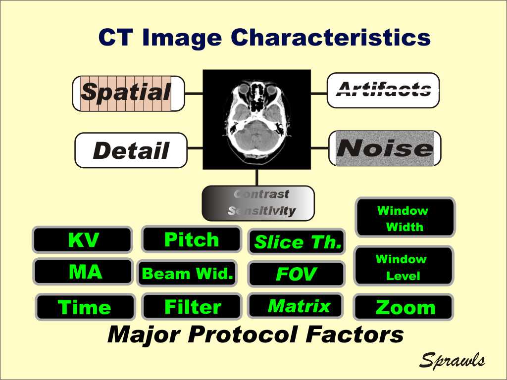
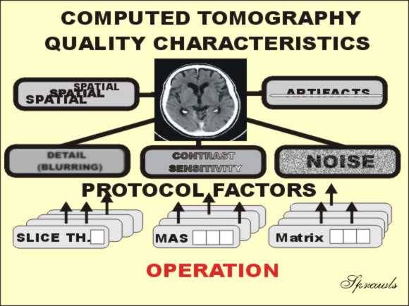
The one comprehensive CT
image quality characteristic is visibility. That is the visibility
of anatomical structures, various tissues, and signs of pathology.
However, visibility depends on a somewhat complex combination of the
five (5) more specific image characteristics shown here.
Each of these can have an effect on the visibility of specific anatomical or pathologic objects within the body. Now the important point is that each of these characteristics is generally adjustable and can be changed or set by a combination of the protocol factors. The challenge is it is not a "one-to-one" relationship. One protocol factor (such as slice thickness) has an effect on both detail and noise. It is this complex combination of protocol factors that will make up an optimized procedure that we will now be working on. |
|
All of the image characteristics are important and have a
potential effect on visibility but the characteristic, contrast
sensitivity, is especially significant in CT because it is what makes it
a superior imaging modality for many clinical procedures. The
concept of contrast sensitivity is illustrated here. With CT imaging the principle source of physical contrast within a body are the differences in physical density among the tissues. An exception is when an iodine-based contrast medium is used where it becomes more of an atomic number (Z) effect.
Compared to other x-ray imaging modalities CT has a very
high contrast sensitivity for "seeing" the soft tissues and differences
among the tissues in the body. How this is produced and controlled
will be illustrated later. Within a body there will be tissues and objects with a range of densities and physical contrast. As illustrated here things like bones, bullets, and barium have a very high physical contrast relative to the soft tissues. Imaging them is not a problem. The real challenge is imaging the very low density differences between and among the soft tissues. That is where CT excels! Contrast sensitivity determines the range of visibility with respect to physical contrast. If a procedure has low contrast sensitivity then only objects with high physical contrast will be visible. When a procedure, such as CT, has high contrast sensitivity then tissues with small differences in density will be visualized. If the contrast sensitivity is low, either because of limitations of the specific imaging modality or the adjustments of the imaging protocol factors then tissues that have small differences in density (physical contrast) will not be visible. |
|
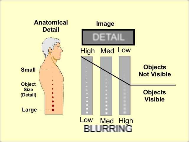
A characteristic of all imaging methods, including human
vision, is that there is some blurring that occurs within the process.
The effect of this blurring is that it reduces visibility of detail
(small objects and features). When we have blurred vision we can't read
the fine print. Each medical
imaging method has inherent sources of blurring that limits visibility
of detail and determines the types of diagnostic procedures it can be
used for. For example, radiography which has relatively low blur
and provides high visibility of detail is used for visualizing small
bone fractures.
The general relationship of detail to the blurring
within the imaging process is illustrated here.
As the blurring increases more and more of the small objects become invisible. In the CT imaging process there are several sources of blurring that collectively limit visibility of detail. There are adjustable protocol factors associated with each of these sources of blur as we will soon see. Now that brings up and interesting question, If we can adjust the blurring why not set it to a low value and get very high visibility of detail? The problem is when we reduce the blurring it increases another undesirable image characteristic, visual noise, and can also lead to increased radiation dose to the patient. That is why we must have optimized imaging protocols that take all of these factors into account and provide a proper balance. |
|
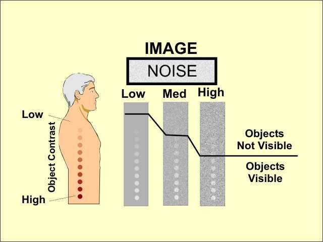
All medical imaging methods produce images with some visual noise.
This is generally an undesirable characteristic that reduces visibility
of certain types of objects and structures as illustrated here. Specifically, noise reduces the visibility of low-contrast objects. This is especially significant in CT which is often used to image low-contrast differences among tissues. Let's take a moment to distinguish between noise and blurring. Both are characteristics that reduce visibility, but of different types of objects. Noise reduces visibility of low-contrast objects, blurring reduces visibility of small objects or detail. The noise in a CT image can be adjusted with a combination of protocol factors. So, why don't we adjust it to a low value and have great visibility? The challenge is that the factors that
can be used to adjust and reduce noise also have an effect on either
image detail (blurring) or radiation dose to the patient. That is why we must have optimized imaging protocols that take all of these factors into account and provide a proper balance.
|
|
The spatial and geometric characteristics of a CT image
play a major role in optimizing the imaging protocols. That is
because the CT image is made up of many small elements or voxels as
illustrated here.
It is the size of the voxels that has a major impact on image blurring, noise, and on radiation dose to the patient. The size of the voxels is controlled by a combination of the three protocol factors shown here.
|
|
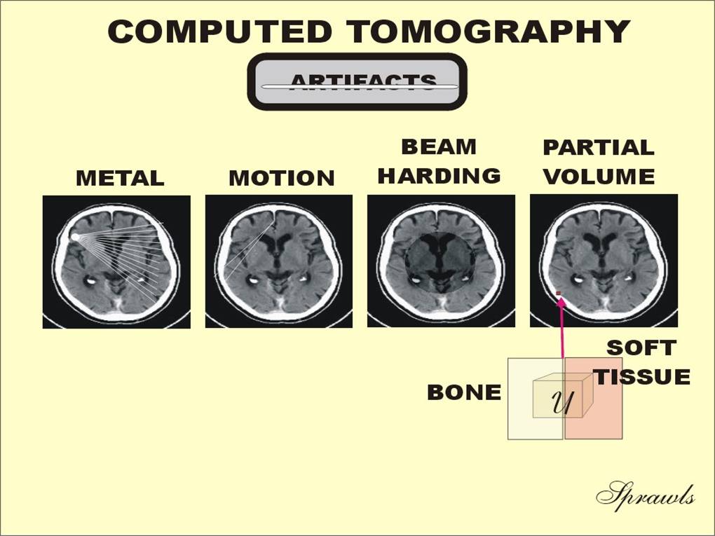
We finish our introduction to the five CT image characteristics with
artifacts. Some possible CT artifacts are shown here.
There are quite a few possible artifacts coming from a variety of conditions that can occur during an imaging procedure. Some are very obvious such as streaks and "ghosts" while others are less visible but more in the form of changes in how certain areas or objects are displayed.
With the advances in CT technology many artifacts are
less common. The most effective approach to learning CT artifacts
is through their observation and analysis while viewing clinical images.
|
|
Now is is time to associate the image characteristics
that we have introduced to actual CT images.
We can compare each to the reference image shown at the bottom and identify the characteristic that makes it different. Based on what we have learned up to this point, make a note of the characteristic that you think makes A, B, and C different from the reference. Now go on to NEXT to see how your answers compare.
|
|
In the first we see a difference in contrast.
Differences in image contrast like we see here are generally the result
in different adjustments in the contrast sensitivity of the imaging
procedure. In CT that is the window level and width control, but
more on that later. When we look at the center image we see that it is blurred and visibility of detail is reduced. In this illustration the blur is abnormally high (to make the point!) but there is some blur in all CT images that must be taken into consideration, both because of its effect on visibility and that it is adjustable. The image on the right shows us what noise looks like. It too must be taken into consideration. Now it's question time again! Image quality is related to radiation dose in several different ways as we will be learning. Comparing each of the three images to the reference image, how do you think they compare with respect to radiation dose?
|
|
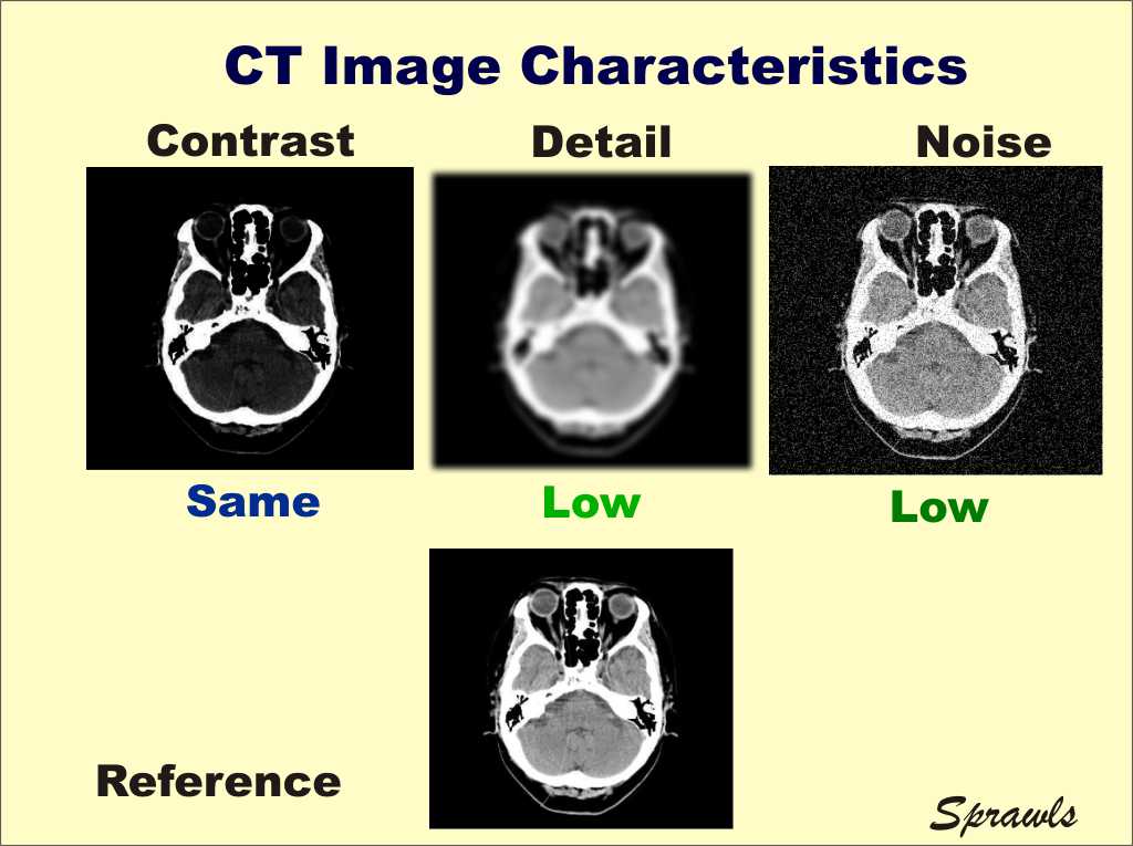
The point being introduced here is that there is a
significant relationship between CT image quality characteristics and
the radiation dose required to produce the image.
Our question was how do we think the dose compared to the reference for our three images.
Generally, in CT image contrast or
the contrast sensitivity of the procedure does not have a
significant dependency on dose. This is Image noise is a major factor in determining dose to the patient. An increase in dose is required to reduce dose as we will see later. In this illustration we have an image with relatively low detail, or is blurry. The dose to produce it would have been lower that the dose to produce the higher quality reference image at the bottom. The very important issue of optimizing a CT imaging protocol involves producing a balance among image detail, image noise, and the dose to the patient. That is what we will do now.
|
|
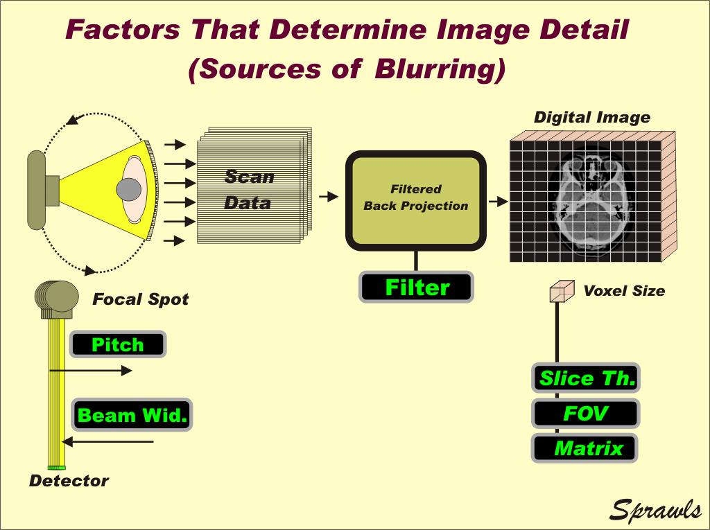
The The first phase is the scanning of the x-ray beam around and along the patient's body and the collection or acquisition of the data. This produces the scan data (but not yet an image) that is stored in the computer memory. The second phase is the image "reconstruction" from the collected data. This results in a digital image of the individual slices or 3D volumes The third phase is the conversion of the invisible digital image into a visible (analog) image for display and viewing. There are several adjustable factors that can be used to optimize the displayed image for a specific clinical task.
|
|
In the scan phase there are two distinct motions of the x-ray beam relative to the patient's body as shown here.
One is the rotation of the x-ray tube and x-ray beam around the body to produce many different "views" thought the body. The other is scanning along the length of the patient and is achieved by moving the body thought the scanner while the beam is rotating around it. It is the combination of these two motions that produce the complete set of data from which the images can be reconstructed.
|
|
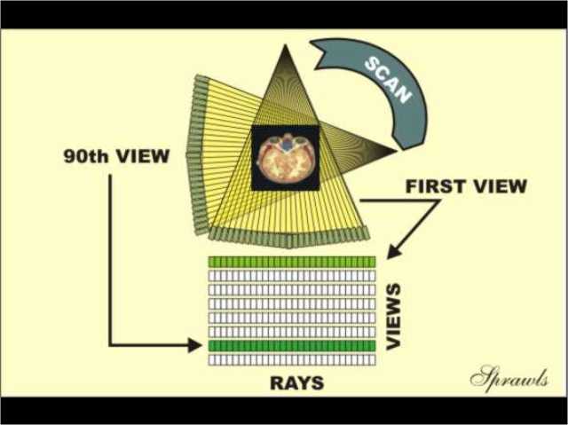
F
From each x-ray tube position it typically projects a thin, fan-shaped beam through the patient's body. After passing thought the body the beam in intercepted by an array of radiation detectors. The pathway from each x-rat tube focal spot position to each detector element is designated as a ray. The detector measures the radiation that penetrates the body along each ray and records it as one data point. As the x-ray tube is scanned around the body it produces views from each position, typically about every one degree of angle. One complete scan around the body produces several hundred views. Data from these many views are required to produce a high-quality image for each slice. The data set to produce an image of one slice is made up of the measurement of each ray in each view. A very large quantity of data! |
|
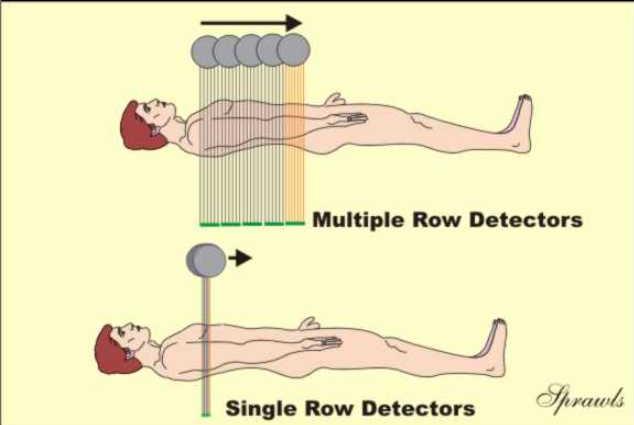
Most CT scanners have detector arrays consisting of multiple rows
compared to the single row detectors that were common in the past.
A design characteristic of a scanner is the number of detector rows (16, 32, 64, etc). A fan-beam scanner has approximately the same number of rows as number of detector elements in each row.
|
|
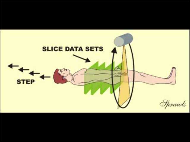
In order to form or reconstruct an image of a specific
anatomical slice or volume there must be sufficient scan data for that
part of the body.
The simplest, and the only method available for many years is the "scan and step" method illustrated here. With the body not moving the x-ray beam is rotated completely around the body and a data set for a slice is collected. With this method the data set is "locked" to a specific slice determining its thickness and position. After each beam rotation the body is then moved or "stepped" to the next slice position where it is scanned. The two major limitations of this method are that it is relatively slow in covering a body section and the slices (position and thickness) are fixed at the time of the scan and cannot be changed later.
Spiral or Helical Scanning
If we can imagine the path of the x-ray beam on the patient's body it would form a spiral or helical pattern. Either name is an appropriate description of this method. There is one very important adjustable protocol factor associated with this method that can have an effect on both image quality and dose to the patient. That is the Pitch factor which is the distance the body is moved, as a multiple of the beam width, during one rotation of the x-ray beam. For example, if the pitch is set to a value of 2, the body would be moved twice the thickness of the beam during on rotation Increasing the pitch value increases the relative speed of moving the body and reduces the time required to cover an anatomical area. We will come back to this in more detail later but in general increasing pitch reduces the dose to the patient but can limit image quality. A very significant value of
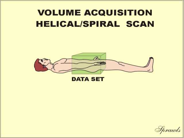
spiral/helical scanning is the characteristics of the data set that is
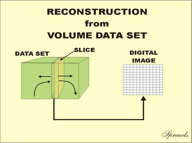
produced as illustrated here. The data set is continuous over the anatomical area scanned and not divided into individual slices as with the scan and step method described above. This offers much flexibility when the images are being reconstructed. With the continuous data set it is possible to reconstruct images of slices anywhere within the data set. These images can be reconstructed for different slice thicknesses and orientations. With spiral scanning the slices are
determined at the time of reconstruction, not at the time of the
scanning and data collection. Another great value of helical scanning is that the continuous data set can be used to reconstruct 3D or volume (compared to slice) images. |
|
CT image reconstruction is a mathematical process for
converting the scan data into a digital image of a specific anatomical
area. Most images are created with the filtered back-projection
method or sometimes with an enhanced process generally known
(generically) as iterative reconstruction.
Voxels
The voxels in the slice of tissue are generally
represented by pixels (picture elements) in the reconstructed digital
image.
|
|
Let's continue to develop the relationship between the tissue voxels within the slice and the pixels in the image. Let's recall that during the scanning phase the individual rays of the x-ray beam are projected through the patient's body. They are attenuated (absorbed) in proportion to the attenuation properties of the tissue along the path. This property is represented by the value of the attenuation coefficient for the specific tissue. Because of the characteristics of the x-ray beam used in CT (high KV and heavy filtration) the attenuation is highly dependent on tissue density. During the back projection reconstruction process the attenuation coefficient value of each individual voxel is calculated. However, we never see the actual attenuation coefficient values because there is another step in the mathematical process performed by the computer. A CT number value is calculated from the attenuation coefficient value for each voxel and becomes the value for the corresponding pixel in the digital image. The formula for this calculation is shown in the illustration. Water (H2O) is used as the reference and calibration material for CT numbers. Water has the assigned CT number value of zero. Tissues or other substances that are more dense than water will have positive (+) values and those that are less dense will have negative (-) values. CT numbers calculated in this matter are in Hounsfield units, named for Sir Geoffrey Hounsfield, the engineer who invented and developed computed tomography.
|
|
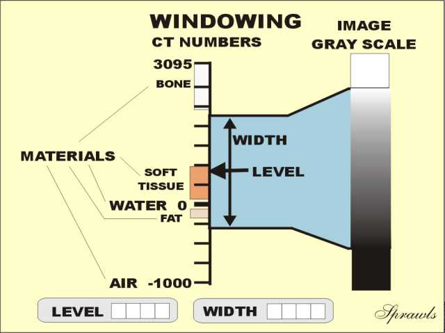
The CT numbers in Hounsfield Units, with water at the zero (0) point, range from negative (-) 1000 for air to plus (+) approximately 3000 for dense bone. Since CT number values are strongly related to tissue densities the various tissues and materials are distributed along the scale according to their density. It is this difference in densities that is the source of the physical contrast that will be converted and displayed as visible contrast in the images. To a great extent, the very high contrast sensitivity of CT is derived from the the ability to select a small range of CT numbers and display them over the full brightness range (dark black to bright white) in the image. This occurs during the third phase of the process and can be controlled by the person viewing the image. The range of CT numbers to be displayed in the image is designated as the WINDOW. The two adjustable protocol factors that control the window are the LEVEL and the WIDTH. The LEVEL control sets the midpoint of the window range along the CT number scale. It can be used to optimize the image contrast for viewing different anatomical regions. A relative low window might be used for seeing the contrast within the lungs and a high window to see contrast within bones. The WIDTH setting is very much of an image contrast control. Reducing the window width increases the contrast among tissues as they are displayed in an image. |
|
There are several issues in selecting and adjusting an optimized protocol for a specific clinical objective. The first priority is adjusting the image characteristics to provide visibility of the anatomy or pathological conditions of interest. We have already introduced the five (5) individual image characteristics that collectively have an effect on visibility. We will soon see how they can be controlled. The overall goal of an imaging procedure is to produce images that have the quality characteristics required for the clinical objectives and to keep the radiation dose to the patient as low as possible without jeopardizing the required image quality. Optimizing a CT protocol is the rather complex process of balancing the image quality characteristics both among themselves and with radiation dose. That requires a knowledge of both the science, especially physics, and the evolving technology that is being used. Our next step is to see how the radiation dose to patients is described and determined. |
|
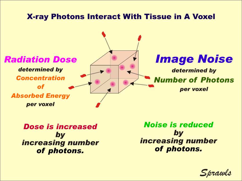
Let's begin with a review of the concept of radiation dose. It is defined as the concentration of radiation energy absorbed in a specific tissue location within the body. The most common unit for expressing dose values is the grey (G) defined as the absorption of a joule of energy per kilogram of tissue. We emphasize that dose is the concentration of absorbed energy at each point in the body. That is, there is a dose value for every point or location within the body. What makes the determination and description of dose for a specific patient very difficult is that the radiation is unevenly distributed throughout the body as the x-ray beam is scanned around and along the body. Another quantity that is sometimes used is the total radiation energy absorbed in the body without regards to the anatomical location. Each, absorbed dose and total radiation energy, has its place in expressing relative risks to patients. We will now continue developing the methods for determining the dose to a patient.
|
|
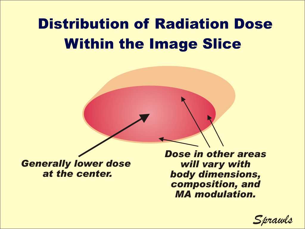
A major factor
contributing to the complexity of determining the dose for a specific
patient in the variation in distribution both within a slice and also
along the length of the body.
Within the plane of each slice there is variation in the dose because of the shape and size of the body and internal composition. The variation can be different for heads compared to the larger sections of the body. In general, the dose is usually somewhat lower at the center of the body.
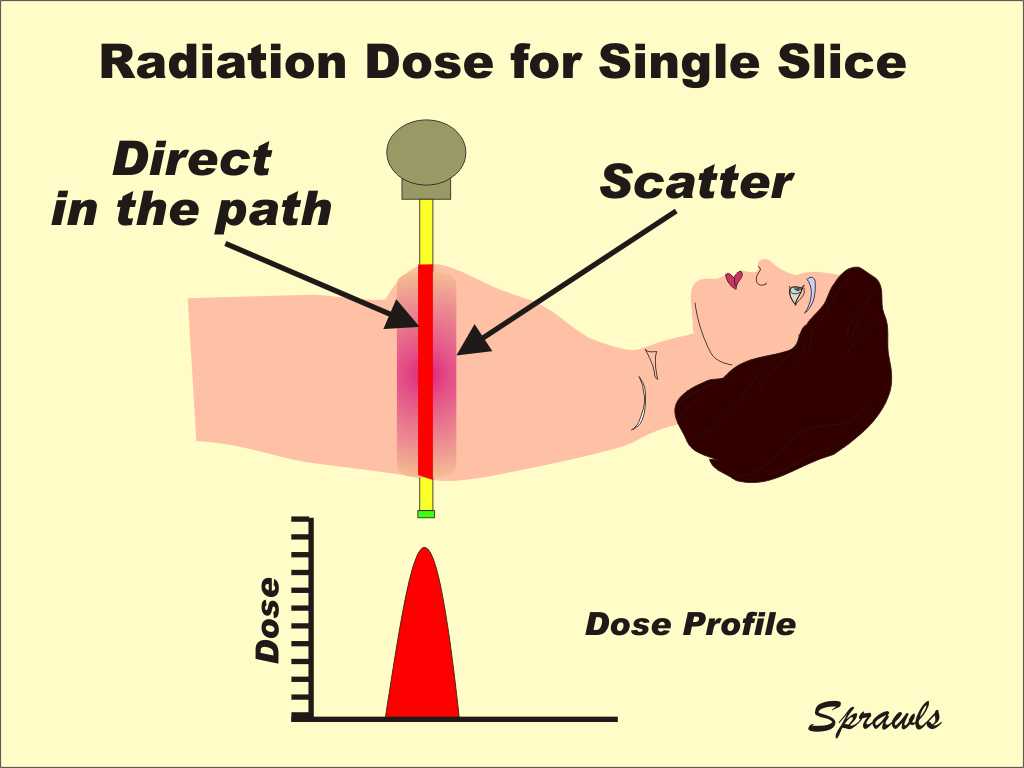
Now let's consider the distribution of
dose along the length of the patient by
Most of the dose is deposited in the slice that is being scanned but there is also some radiation that scatters out of the slice and produces some dose in the adjacent tissues. This scattered radiation complicated the process of determining the dose when more that one slice is imaged as in the usual procedure. An additional complication is the fact that we cannot place instruments, or dosimeters, directly into the body to make measurements. Because of this combination of factors and challenges the dose values for a specific patient are are determined or estimated through a series of external measurements and calculations. |
|
Because it is not practical to measure directly the dose deposited in a patient's body an indirect, and somewhat complex process is used. We will now go thought that process which takes into account some of the variable factors that must be considered.
The first step is to measure the dose in a phantom that represents a patient body. The typical phantom is an acrylic cylinder that has the same x-ray absorption properties as soft tissue. It is described as being a "tissue equivalent" material with approximately the same density and effective atomic number (Z) as soft tissue. A smaller phantom is used to represent a head and a larger one for the abdominal section. A dosimeter, typically an ionization chamber, is placed in the phantom and a one-slice scan is performed and the dose measured. Now to consider the first problem. As we observed earlier some radiation scatters out of the scanned slice and exposes the adjacent tissue. This becomes significant in the typical scan which consist of many slices. The question (?) is "what is the dose within one slice" from both the direct x-ray beam through the slice and the scatter from other slices? The problem is we do not have any practical method to measure the dose in any one slice when it is within the midst of other slices that would expose the dosimeter to their direct radiation. Now for the solution...it has been demonstrated that if a dose measurement is made for just one scanned slice the scattered radiation out of the slice and measured by the dosimeter will give a good approximation to the dose within a slice including the scattered radiation from adjacent multiple slices. Since this is not an actual direct
measurement, but an indirect approximation, under multiple slice
conditions it cannot correctly be referred to as "dose". The value
measured by this process and used as an estimate of the actual dose is
designated as the: Therefore, CTDI values, and not actual dose values, are used to describe the radiation to patients. Now for the next step.
|
|
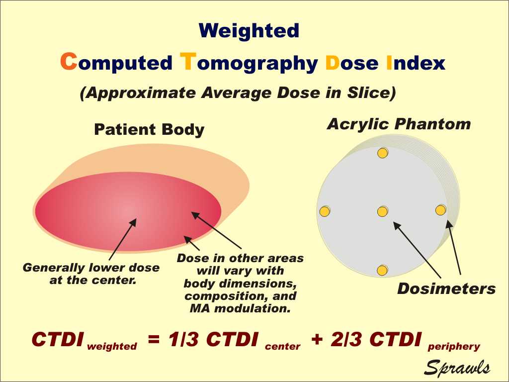
As we continue with the process of
determining and expressing the radiation dose to a patient the next
factor to consider is the variation in dose values within the plane of a
slice as described before. To account for this the usual procedure is to use a phantom with five (5) dosimeters. The five measured values are then used to calculate a "weighted" value using the formula shown here.
|
|
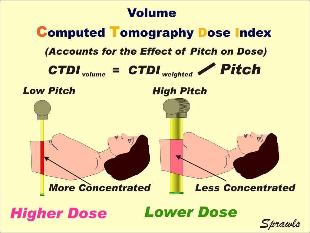
Now to take into account another factor,
the effect of pitch on dose. We have already introduced the adjustable protocol factor, pitch, as having an effect on how fast the body is moved through the x-ray beam. Since dose is the concentration of radiation absorbed in tissue, increasing the pitch value with all other factors remaining unchanged "spreads" the radiation and makes it less concentrated. The dose becomes inversely proportional to the pitch. The volume CTDI is determined by dividing the weighted CTDI by the pitch and provides an estimate of the dose for specific pitch values used in spiral scanning.
|
|
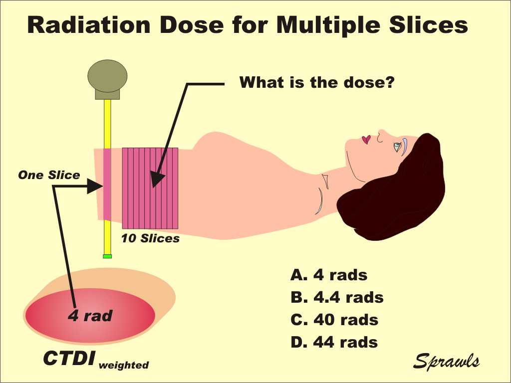
The CTDI as we have developed up to this
point provides an estimate of the dose within individual slices. Now let's think about the dose when multiple slices are scanned. Here we have a question based on this illustration. If the CTDI within a single slice is 4 rads what is the dose if 10 slices are scanned? Notice that four possible answers are given. What is your choice: A, B, C, or D? ____________________________________________ The important point to remember is that "dose" is a quantity that expresses the concentration of radiation energy absorbed at a specific point within the body. Scanning multiple slices does not multiply the concentration within the individual slices, it does deposit radiation energy (dose) in additional slices. With multiple slices there is some, but relatively small, increase in the dose to a slice by the scattered radiation from adjacent slices. This is probably in the range of 10% - 20%, depending on specific conditions. Does that help you select the best answer? If scanning multiple slices DOES NOT multiply the dose within the slices, what is its major effect? It increases the total radiation energy deposited in the body, but not the concentration in any of the slices, except for the scatter contribution. Our next step is to come up with a
quantity that can be used to express the relative amount of total
radiation to the body.
|
|
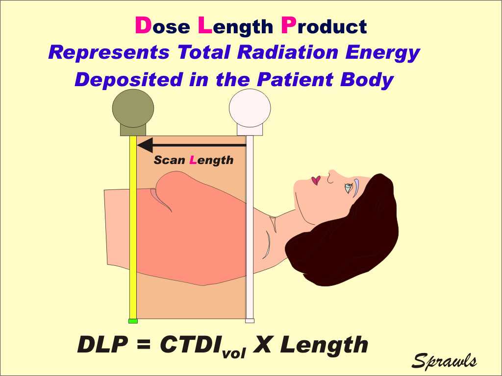
The total radiation energy deposited in a patient's body
can be estimated by multiplying the dose within a slice by the distance
(length) scanned along the body as illustrated here. The advantage of DLP is that it is relatively easy to determine for each patient scan. Many scanners can automatically calculate it and display the value as part of the patient information. There are two ways that DLP values can be used. They can be used to compare various scanning protocols with respect to the total energy imparted to a patient. Since this is not an actual energy unit it provides a relative comparison only. DLP values when combined with other factors can be used to calculate the effective dose to the patient. That is our next step.
|
First, a quick review. Let's recall that effective
dose is the quantity that is used to estimate relative risk to a patient
taking into account the distribution of dose values to the various
organs and anatomical regions and the relative sensitivity of the
different tissues as quantified in terms of the values for the tissue
weighting factors.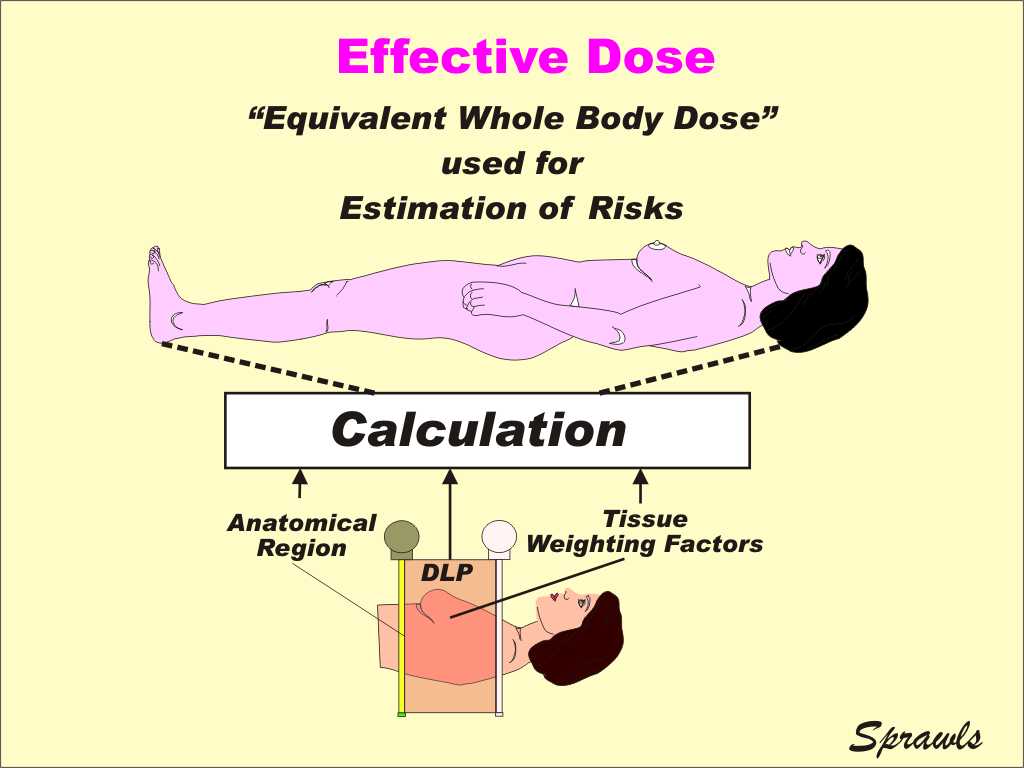 The value calculated for effective dose is generally assumed to have the same detrimental biological effect as a dose of that value to the whole body. The effective dose for a CT scan can be calculated from a DLP value using tabulated data of the tissue weighting factors for the organs within the scanned area. Effective dose values are generally used to compare the relative risks of various CT imaging protocols. Also, effective dose values are used to compare a CT procedure to normal background radiation which is a whole-body exposure. |
|
We are almost there! Our goal is to determine a
dose value for a patient undergoing a CT procedure. As we have
observed, there are a variety of factors that must be considered and
several different quantities associated with the factors and conditions. The first step, usually performed by a physicist, is to measure the weighted CTDI in a phantom. This provides basic calibration data for the scanner. By using the KV, Time, and MA values for a specific patient and the calibration data the weighted CTDI for the patient can be calculated. The next step is to use the pitch value (spiral/helical scanning) to calculate the volume CTDI. This is often calculated and displayed by the scanner as part of the patient information. Multiplying by the length of the scan provides a value for the DLP, the relative total energy imparted to the body. This is also calculated and displayed by many scanners. The final step is the calculation of the effective dose that provides an estimate of the relative biological effect on the patient.
|
|
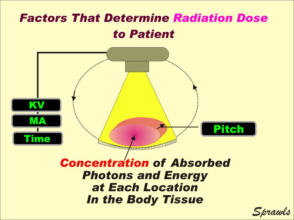
Up to this point we have covered two major areas. First we were introduced to the individual image characteristics that have an effect on visibility and overall image quality: contrast, blurring, noise, spatial (geometric), and artifacts. Then we worked through the various radiation
quantities used to express radiation delivered to a patient and the
factors that must be taken into consideration to find actual values. The next big and important step is relating radiation dose to image quality. That provides us with the background for optimizing imaging protocols and producing images with the necessary clinical quality without unnecessary radiation dose. The actual dose to a specific anatomical location is generally determined by the values selected by the operator for the protocol factors shown here and the size of the patient. In principle, the dose can be reduced by setting the KV, MA, and Time to lower values and increasing the pitch. So the obvious question what is to prevent us from doing it? The answer...changing these factors to reduce dose will also have a significant effect on image quality. That is why an optimized protocol is one in which the factors are selected to produce an appropriate balance between image quality and dose. It becomes somewhat complex because we must also develop a balance between two of the image quality characteristics, (detail) blurring and noise. That's where we go now.
|
|
We will begin by considering the adjustable protocol
factors that control image detail as shown here.
The ultimate detail available in an image is determined by the total effect of the blurring that occurs throughout the image formation process. The most significant blurring occurs in the first two phases, scanning and reconstruction. We call that in the scanning phase the x-ray beam is divided into many small rays that pass through the body and measure the attenuation along their path. For good detail (low blurring) we must scan with small rays. The size of an individual ray is determined by the size of the focal spot on one end and the size of the detectors on the other end. The dimension of the ray that is usually variable is the beam width which is determined by the number of detector elements selected in that dimension. Increasing the pitch has the effect of "spreading" the ray and introducing blurring along the length of the body. Important point....if an image with high detail is required "high detail" scan data must be collected, generally by scanning with a thin beam and low pitch value. An image with high detail cannot be reconstructed later if the "detail" is not in the scan data. During the reconstruction phase there are two additional sources of blurring that adds to the blurring in the scan data. One is blurring that might be produced by the mathematical filter in the reconstruction calculation and the other is the size of the tissue voxel. We will work with each of these after we bring noise back "into the picture".
|
|
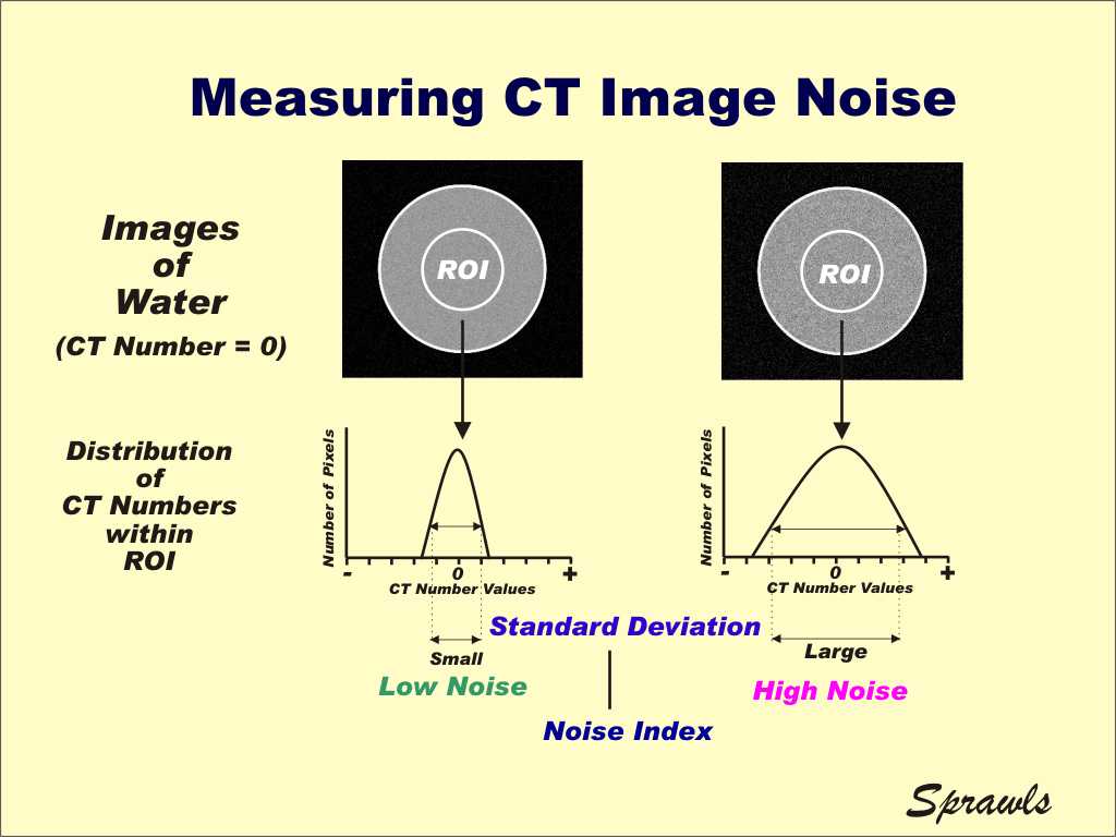
The measurement of CT image noise is a
relatively easy and routine process as illustrated here and it helps us
understand the characteristics of noise and an introduction to how it
can be controlled. CT image noise is a form of "quantum noise" that is found in all types of images formed with x-ray or gamma photons. The noise that we see is actually an image of the natural random distribution of the photons over the image area. To see and measure the noise we scan and produce an image of something that is completely uniform with one CT number throughout and has no objects or structures in it, as a human body would have. A container of water (often called a phantom) is ideal for this purpose. Here we see two images that have different amounts of noise. The one on the left is less than the one on the right. The measurement is made using the CT system from the viewing console. Using a standard viewing function a region of interest (ROI) is selected within the image. The next step is to use another standard function of the CT system which measures the statistical standard deviation of the CT numbers (pixel values) within the ROI of the image. Water has a theoretical CT number value of zero (0) Hounsfield units. That is the value all pixels would have in a perfect image WITHOUT any noise. The effect of the noise in a CT image is to cause a statistical variation in the actual CT numbers from pixel to pixel. The range of this variation, as measured by the calculated standard deviation (SD), is a measure of the noise. This is often referred to as the noise index. We see that the image on the right has more visual noise, a greater variation in CT number values, and a larger calculated SD value. This now leads us to a very important question, "why does the image on the right have more noise"?, and can we do anything to control or reduce it?
|
|
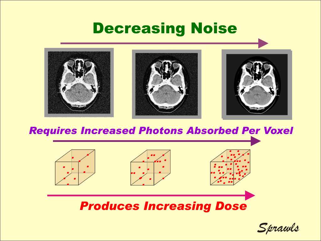
The noise in an image comes from statistical errors
in the measurement of the CT numbers of each tissue voxel.
The precision of measurements made based on the number of photons that are attenuated or absorbed depends on the average (mean) number of photons involved. The precision increases (the error and noise decreases) as the number of photons used is increased. Let us recall that the standard deviation (SD) is inversely related to the average or mean of the number of the photons in each measurement. In this case it is the number of photons absorbed in each voxel. While we can easily reduce the noise by "turning up" the exposure and increasing the number of photons that has the undesirable effect of increasing the radiation dose to the patient. That is one of the issues we must address in our effort to provide an optimized imaging protocol for each patient. The goal is to get a sufficient number of photons absorbed in each voxel while keeping the absorbed energy (dose) as low as possible.
The important point here is the difference between the
number of photons absorbed in each voxel and the concentration of
photons absorbed which determines the dose. This can be achieved by increasing voxel size. A larger voxel will capture more photons without affecting the dose.
|
The individual voxels are formed during the
reconstruction phase and their size is controlled by a combination of
the three protocol factors shown here.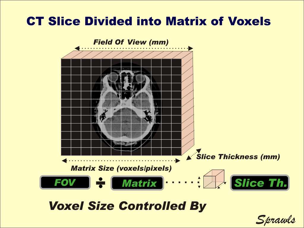 The ratio of the field of view (FOV) to the matrix size (number of voxels across the slice) determines the "face" dimension of a voxel. This corresponds to relative pixel size in the image. Some quick mathematics.... if we have a 25cm (250mm) field of view and a 512 matrix size that gives voxels with a face dimension of 0.5mm. This is an indication of the relative detail available in CT images. The other dimension of the voxel is the slice thickness. It is typically the largest dimension of a voxel and the factor that is often varied the most for different clinical procedures. Now let's consider the issues that must be considered when selecting an appropriate voxel size for a procedure. Do we want a small or large voxel?
This is one of the major factors in optimizing an
imaging protocol because we have to reach a compromise. That is because larger voxels "capture" more photons for a specific dose and that improves the statistics and reduces the noise.
|
|
The noise in an image is determined
by a combination of protocol factors as we see here.
During the scanning phase the same factors we introduced earlier as those that affect dose also have an effect on noise because they control the concentration of photons absorbed in tissue. Changing any of these factors changes both noise and dose. Now to the reconstruction phase. As we have just observed, changing the voxel size changes the ratio of number of photons (noise) to the concentration of photons (dose). The other controlling factor is the mathematical filter that is included in the reconstruction process.
|
|
During the reconstruction process mathematical filters are used to change some of the image characteristics. These might be referred to by different names such as algorithms or kernels but their effects are the same. Each CT system has many different
filters that the operator can select from for a specific clinical
procedure. We are not going into the characteristics of all of the filters here but focusing our attention on their effects of the two image characteristics, noise and detail as illustrated here. Some filters can be selected to reduce noise in an image. However, the reduction of noise by digital image processing usually increases the blurring in the image and reduces the visibility of detail. Filters that are selected to increase or enhance detail typically increase the visibility of image noise. This is all part of the compromise between image detail and image noise. In general noise is reduced by increased blurring (voxel size, filter, etc) but that reduces image detail. That is all part of the process of developing an optimized imaging protocol.
|
|
Let's now look at and summarize all of
the adjustable factors that control detail in a CT image.
We have already considered all of these but need to look at all of them together. Blurring is produced both in the scanning and reconstruction phases. The detail that will be available in an image is limited by the combination of blurring from all sources. If one source of blur is "excessive" it will limit the detail regardless of the other factors. For example, if we scan with a wide beam or high pitch value we cannot overcome this blurring in the reconstruction phase by using small voxels and thin reconstructed slices.
|
|
Another significant issue in optimizing a
protocol is the relationship between image detail and dose to the
patient.
The fact is when we chance factors to increase detail it will generally lead to an increased dose as illustrated here. It is actually a two step and indirect effect. If we change any of the three factors to reduce voxel size to increase detail we also get the undesirable effect of increased noise. That is because smaller voxels capture fewer photons. It would be typical to then increase the MA to decrease the noise, ant that increases the dose. It is this relationship that has often contributed to increased doses in CT. This is especially the case when the staff requires thin-slice and high-detail images without recognizing that the MA is being automatically increased to maintain a specific noise value.
|
|
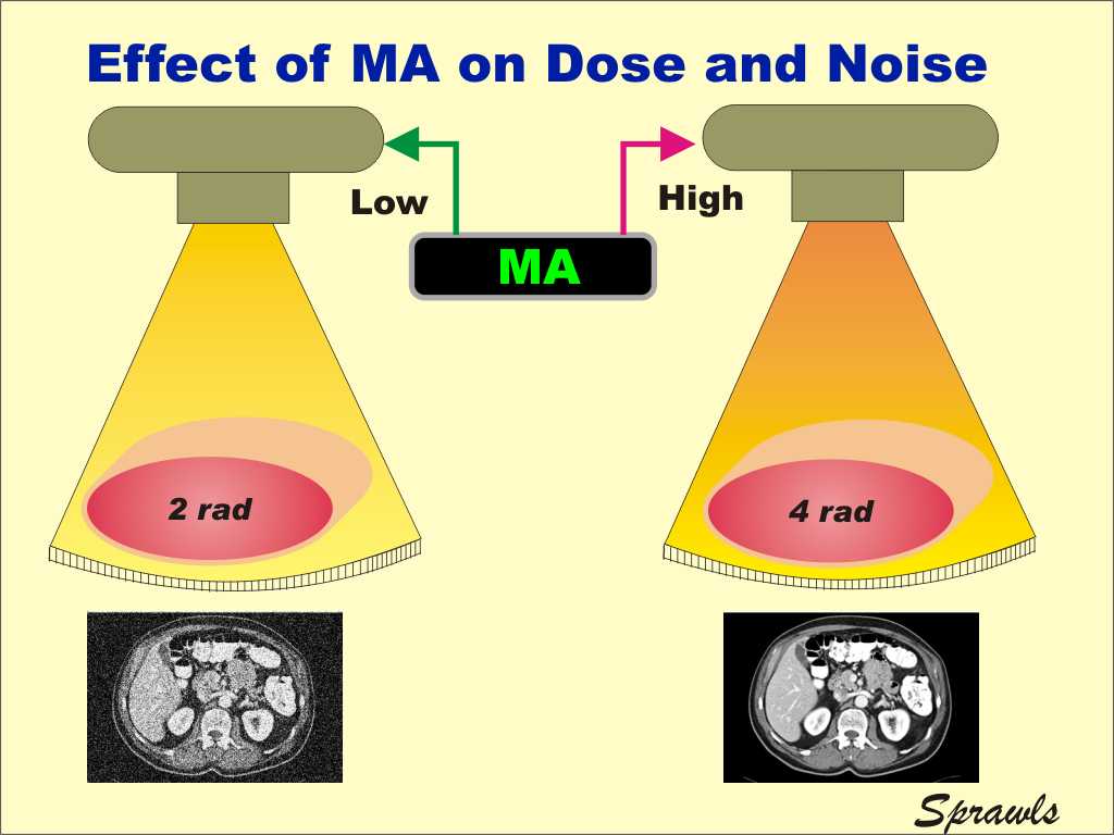
The MA (x-ray tube current) is the
protocol factor that has a direct effect on both dose and noise as we
see here. The general procedure in setting up a scan is to set the MA to a value that will keep the noise to an "acceptable" level. This might be done manually by the operator or by some combination of automatic control functions. It should be recognized that the MA is also controlling the dose. An objective in setting up a protocol is to select a MA value that is appropriate for individual body sizes, shapes, and compositions that will provide a specific noise level without unnecessary dose to the patient.
|
|
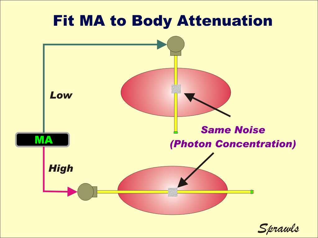
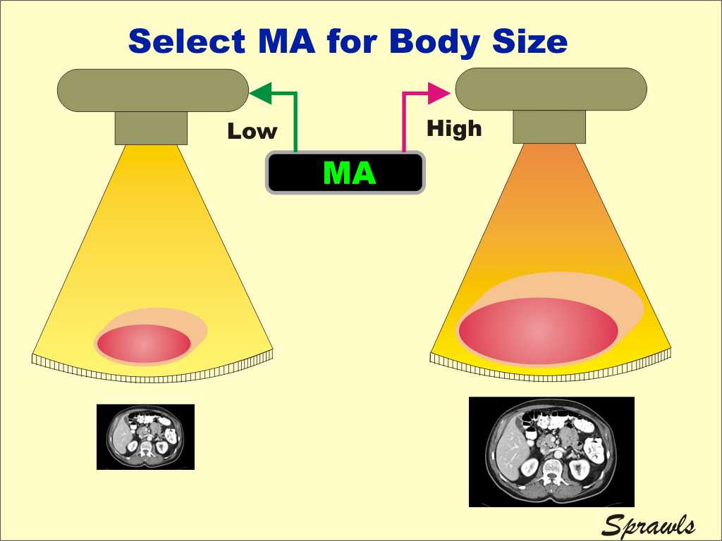
One of the most effective approaches to
preventing unnecessary dose to the patient is to adjust the MA in
relation to the size of the body. For smaller body sizes, with less attenuation of the x-ray beam, a lower MA will produce an acceptable noise level and a reduced dose compared to what is required for larger patients.
|
|
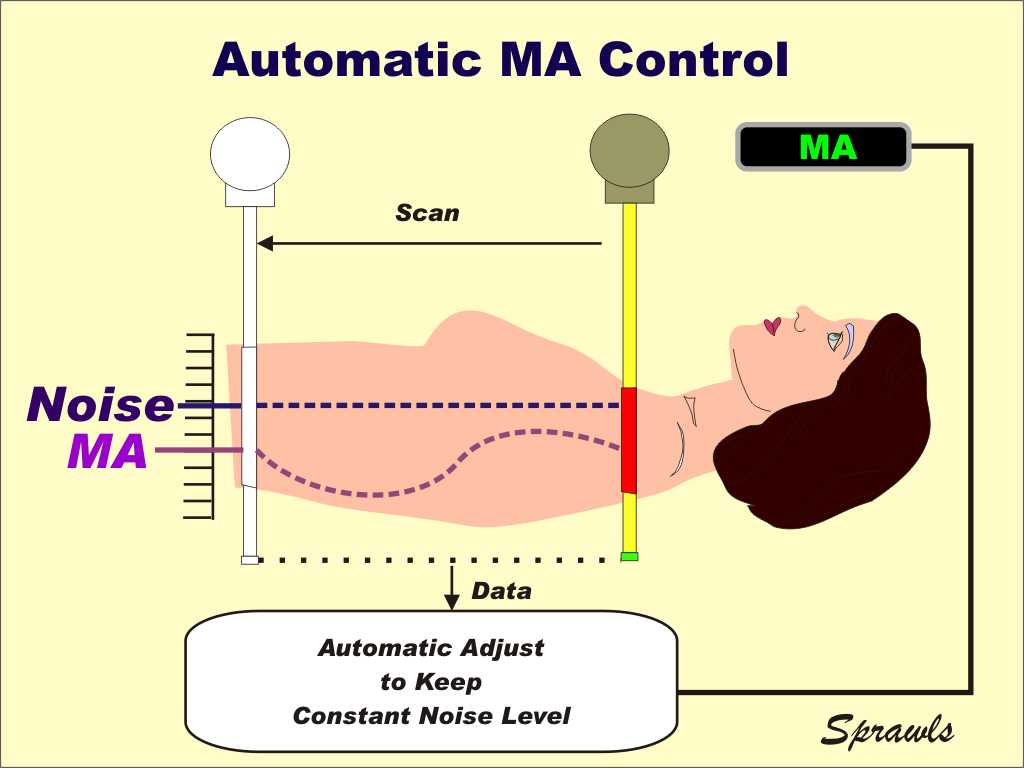
An effective way of optimizing the
dose-to-noise relationship is to adjust the MA for different body
thicknesses and compositions during the scan.
This can be achieved with automatic MA control functions that adjust the MA based on body attenuation thought the body sections. This can include adjustments during the scan of the x-ray beam both around and along the length of the body.
The reference for setting the MA values during the scan is the noise level that will appear in the image. The goal is to maintain a specific noise level without unnecessary exposure to the patient. |
|
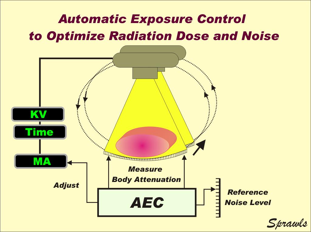
The purpose of the AEC system is to
adjust the MA to account for variations in body size and composition and
maintain a specific level of image noise and image quality. The AEC cannot determine what is the most appropriate and optimum noise level. That is a human function. It is a staff responsibility to have determined the appropriate and acceptable level of noise for different clinical procedures and that is included in the reference noise level settings.
|
|
In this module we have considered how CT
image quality can be controlled through a combination of the various
protocol factors. It is a complex process. With the knowledge of the principles you have obtained up to this point the next step is to become involved in actual imaging procedures. Give special attention to the protocols that are being used for different types of patients and clinical procedures. Consider the quality of the images, especially the noise. Become familiar with the radiation dose values for each patient as displayed with the images. Discuss with other members of the staff the opportunity for improving some of the protocols with respect to image quality and dose. To return to the beginning CLICK HERE.
|
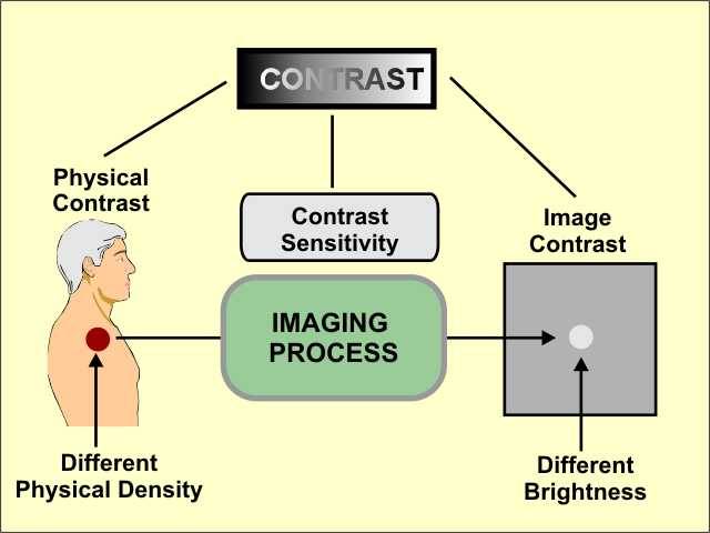 Contrast sensitivity is a characteristic of the imaging process.
That is the capabilities of the imaging equipment (CT scanner) and how
it is adjusted. Contrast sensitivity controls the conversion of the
physical contrast within the body to the visible contrast in an image.
Contrast sensitivity is a characteristic of the imaging process.
That is the capabilities of the imaging equipment (CT scanner) and how
it is adjusted. Contrast sensitivity controls the conversion of the
physical contrast within the body to the visible contrast in an image.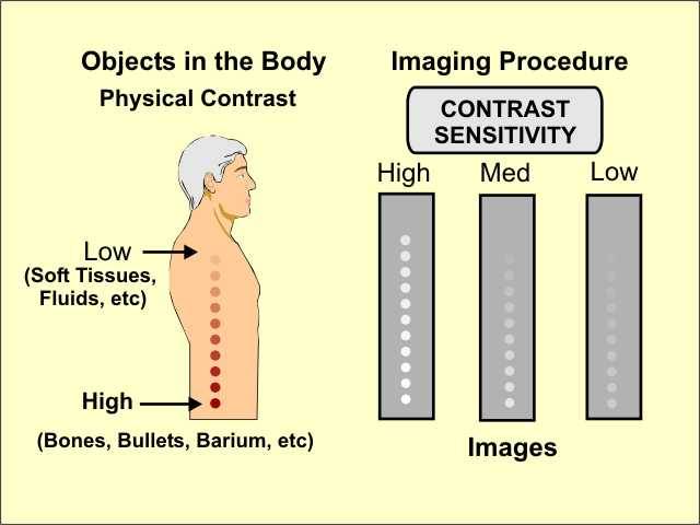
 An
artifact is generally something that appears in an image that is not a
direct visualization of an object or structure in the body.
An
artifact is generally something that appears in an image that is not a
direct visualization of an object or structure in the body.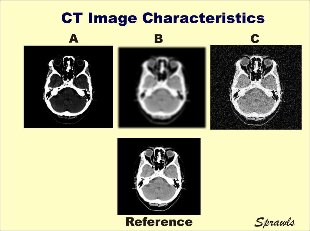 We
will consider the three that have the most direct effect on visibility.
They are:
We
will consider the three that have the most direct effect on visibility.
They are: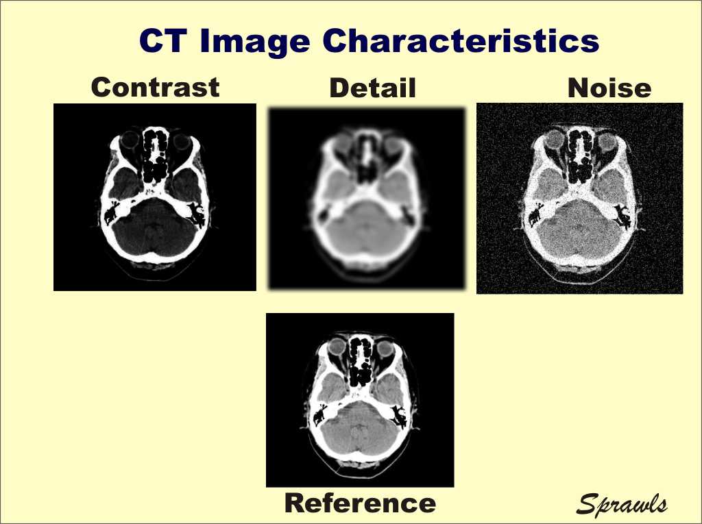
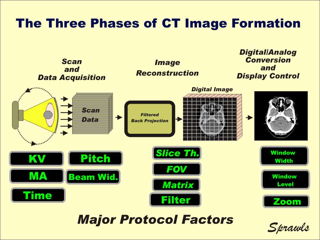 formation of a CT image is a three-phase process as shown here.
There are adjustable protocol factors associated with each phase that
have an effect on image quality and in some cases the dose to the
patient. In this illustration we have identified so of the major
protocol factors that control image quality.
formation of a CT image is a three-phase process as shown here.
There are adjustable protocol factors associated with each phase that
have an effect on image quality and in some cases the dose to the
patient. In this illustration we have identified so of the major
protocol factors that control image quality.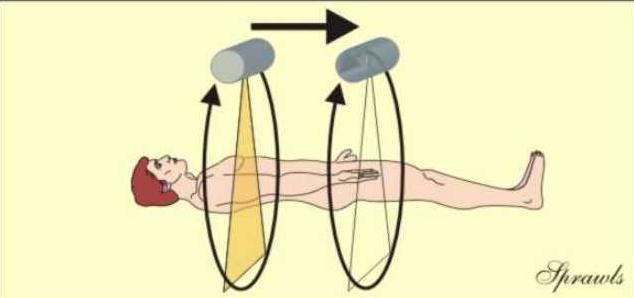
 There
are two distinct methods of scanning the beam along the length of the
body. Each has its characteristics that must be considered.
There
are two distinct methods of scanning the beam along the length of the
body. Each has its characteristics that must be considered.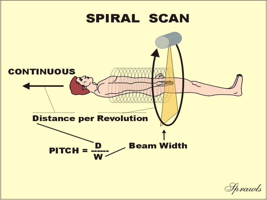
 It is possible to go back and reconstruct images for different slice
characteristics without scanning the patient again.
It is possible to go back and reconstruct images for different slice
characteristics without scanning the patient again.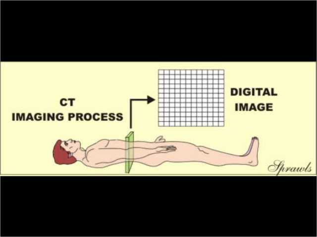 It
is not necessary for us to go into the mathematical details but focus on
sertain characteristics of the reconstruction process that are
adjustable and have an effect on image quality and radiation dose.
It
is not necessary for us to go into the mathematical details but focus on
sertain characteristics of the reconstruction process that are
adjustable and have an effect on image quality and radiation dose.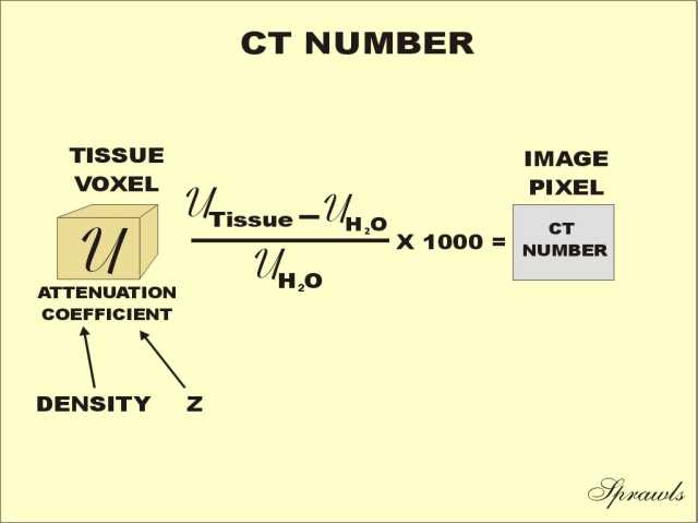
 With
the background that we have developed up to this point let's look at the
"big picture" and see where we go from here.
With
the background that we have developed up to this point let's look at the
"big picture" and see where we go from here.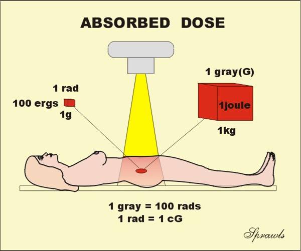
 looking
at the dose for a single slice scan below.
looking
at the dose for a single slice scan below.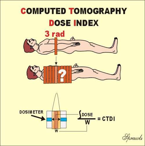

 So the question is how can we increase the number of photons (reduce the
noise) without increasing the concentration of photons and increasing
the dose.
So the question is how can we increase the number of photons (reduce the
noise) without increasing the concentration of photons and increasing
the dose.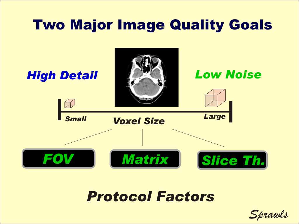 We need to reconstruct images with small voxels to minimize blurring and
get good image detail but increasing voxel size reduces image noise.
We need to reconstruct images with small voxels to minimize blurring and
get good image detail but increasing voxel size reduces image noise.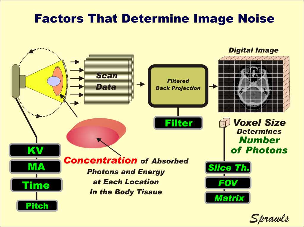
 The filters that are appropriate for the various clinical procedures
have been determined from experience and are typically included in the
established protocols for a facility.
The filters that are appropriate for the various clinical procedures
have been determined from experience and are typically included in the
established protocols for a facility.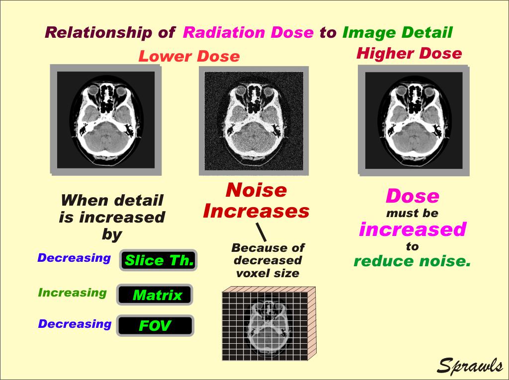
 This is especially important for pediatric patients.