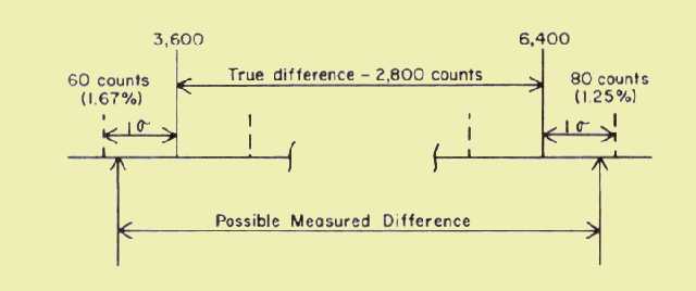
|
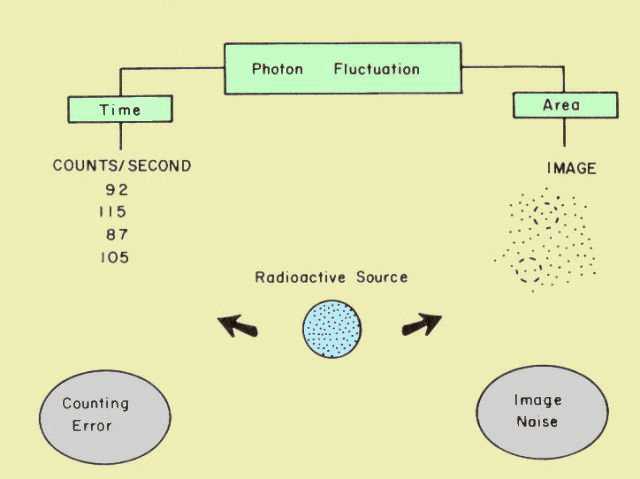
From our
earlier experiment, we know that the value of any individual count falls
within a certain range around the true count value. In our experiment, we
observed that all counts fell within 30 counts (plus or minus) of the true
value (100 counts). Based on this observation, we could predict the
maximum error that could occur when we make a single count. In our case.
the maximum error would be ± 30 counts ( ± 30%). We also observed that
very few count values approached the maximum error. In fact, a large
proportion of the count values are clustered relatively close to the true
value. In other words, the error associated with many individual counts is
obviously much less than the maximum error. To assume that the error in a
single count is always the maximum possible error is overstating the
problem. Although it is necessary to recognize that a certain maximum
error is possible, we must be more realistic in assigning values to the
error itself because it is usually much less than the maximum possible
error.
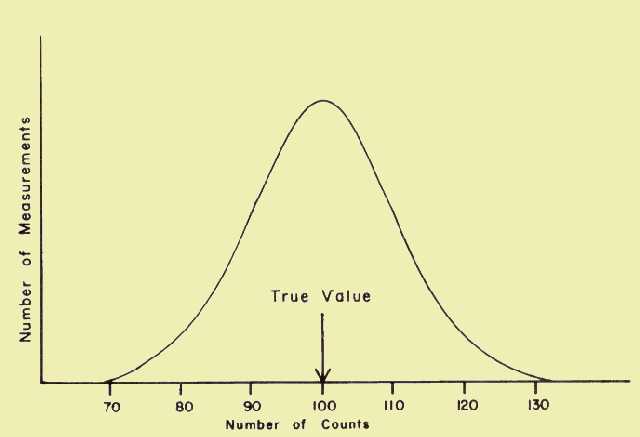
If, at this
point, we were to go back to the data from our earlier experiment and
analyze it from the standpoint of how the individual count values are
clustered around the true value (mean), we would get results similar to
those illustrated in the following figure. For the purpose of this
analysis, we established three error ranges around the true value. In our
particular case, the error ranges are in ten-count increments. The first
range is ± 10 counts (10% error), the second range is ± 20 counts (20%
error), and the largest range is ± 30 counts (30% error). At this point we
are interested in how often the value of a single measurement fell within
the various error ranges. Upon careful analysis of our data, we find that
68% of the time the count values are within the first error range ( ±
10%), 95% of all count values are within the next error range (± 20%), and
essentially all values (theoretically 99.7%) are within the largest error
range ( ± 30%).
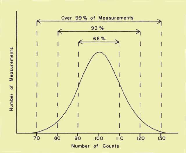
Number of Measurements That Fall within Specific Error Ranges
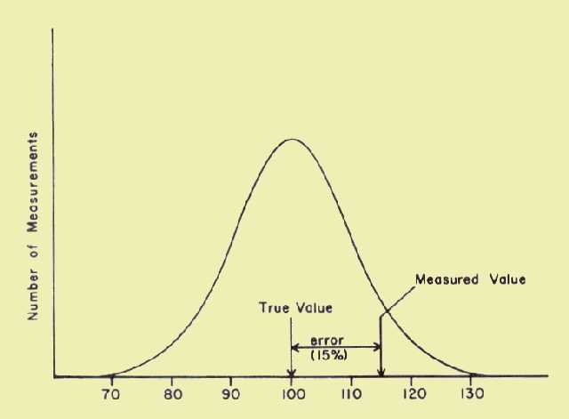
With this
information as background, let us now see what we can say about the error
of an individual measurement. Note that in the case of a single
measurement, there is no way to determine the actual error because the
true value is unknown. Therefore, we must think in terms of the
probability of being within certain error ranges. With this in mind, we
can now make several statements concerning the error of an individual
measurement in our earlier experiment:
• There is a 68%
probability (chance) that the error is within ± 10%.
• There is a 95%
probability that the error is within ± 20%.
• There is a 99.7%
probability that the error is within ± 30%.
While we are
still not able to predict what the actual error is, we can make a
statement as to the probability that the error is within certain
stated limits.
It might appear that the error ranges used above were chosen because
they were in simple increments of ten counts. Actually, they were
chosen because they represent "standard" error ranges used for values
distributed in a Gaussian manner. Error ranges can be expressed in
units, or increments, of standard deviations (s). In our example, one
standard deviation (s) is equivalent to ten counts. However, one
standard deviation is not always equivalent to ten counts.
The general situation is illustrated in the figure which follows the
table below. For values distributed in a Gaussian manner, the
relationship between the probability of a value falling within a
specific error range remains constant when the error range is expressed
in terms of standard deviations. For the general case, we have the
following relationship between error limits and the probability of a
value falling within the specific limits:
Error
Limits
Probability
± 1s
68.0%
± 2s
95.0%
± 3s
99.7%
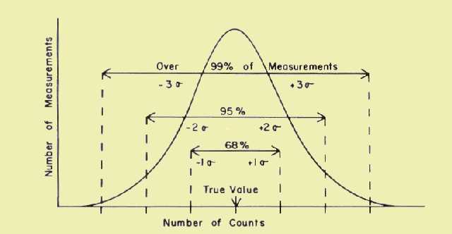
Relationship
between the Number of Measurements within Error Limits When the Limits
Are Expressed in Terms of Standard Deviations
It might be helpful to draw an analogy between the error limits and a
bull's-eye target, as shown below. The small bull's-eye in the center
represents the true count value for a specific sample. If we make one
measurement, we can expect the count value to "hit" somewhere within
the overall target area. Although there is no way to predict where the
value of a single measurement will fall, we do know something about the
probability, or chance, of it falling within certain areas. For
example, there is a 68% chance that our count value will fall within
the smallest circle, which represents an error range of one standard
deviation. There is a 95% probability that the value will fall within
the next largest circle, which represents an error range of two
standard deviations. Essentially all of the values (99.7%) will fall
within the largest circle, which represents an error range of three
standard deviations.
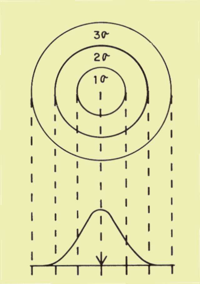
An Analogy between Counting Error and a Bull's-Eye Target
Measuring the relative activity of a radioactive sample is like
shooting at a bull's-eye. We do not expect to get the true count value
(hit the bull's-eye) each time. The problem is that after making a
measurement (taking a shot) we do not know what our actual error is (by
how far we missed the bull's-eye). This is because we do not know what
the true value is, only the value of our single measurement. We must,
therefore, describe our performance in terms of error ranges and the
confidence we have of falling within the various ranges. We can express
a level of confidence of falling within a certain error range if we
know the probability of a single value falling within that range. For
Gaussian distributed count values, 68% will fall within one standard
deviation of the true, or mean, value. Based on this we could make the
statement that we are 68% confident that the value of a single
measurement will fall within the one standard deviation error range. A
more complete description of our performance could be summarized as
follows:
Error Range
Confidence Level
± 1s
68.0%
± 2s
95.0%
± 3s
99.7%
A clear distinction between an error range and a confidence level is
necessary. Error range describes how far a single measurement value
might deviate, or miss, the true count value of a sample. Confidence
level expresses the probability, or chance, that a single measurement
will fall within a specific error range. Notice that as we increase the
size of our error range our confidence level also increases. In terms
of our target, this simply means we are more confident that our shot
will hit within a larger circle than within a smaller circle.
The relationship between confidence level and error range expressed in
standard deviations does not change for measurement values distributed
in a Gaussian manner. What does change, however, is the relationship
between an error range expressed in standard deviations and an error
range expressed in actual number of counts or percentages. In our
earlier example, one standard deviation was equal to ten counts, or
10%. We will now find that for other measurements one standard
deviation can be a different number of counts.
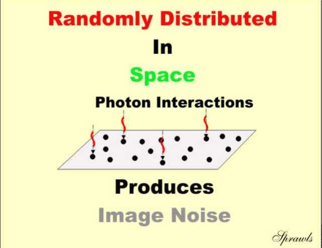
Radiation events (such as count values), unlike the value of many other
non-radiation variables, are distributed in a very special way. The
value of the standard deviation, expressed in number of counts, is
related to the actual number of photons counted during the measurement.
Theoretically, the value of the standard deviation is the square root
of the mean of a large number of measurements. In actual practice, we
never know what the true count value of a sample is. In most cases, our
measurement value will be sufficiently close to the true value so that
we can use it to estimate the value of the standard deviation as
follows:
______________
Standard deviation = √Measured value.
For example, if we make a measurement in which 100 counts
will be recorded, the value of the standard deviation will be
___
s =
√100 = 10 counts.
This will be recognized as the count value in our earlier
example, where it was stated that the value of one standard deviation
was 10 counts, or 10%. Now let us examine the values of one standard
deviation for other recorded count values shown in Table 1. Examination
of this table shows that as the number of counts recorded during a
single measurement increases, the value of the standard deviation, in
number of counts, also increases; but it decreases when expressed as a
percentage of the total number of counts. We can use this last fact to
improve the precision of radiation measurements.
|