
Chapter 5
The Imaging Process
|
|
Chapter 5 |
| Link to Book Table of Contents | Chapter Contents Shown Below |
|
Figure 5-1. The two functions,
acquisition and
reconstruction, that make up the MR image production process. |
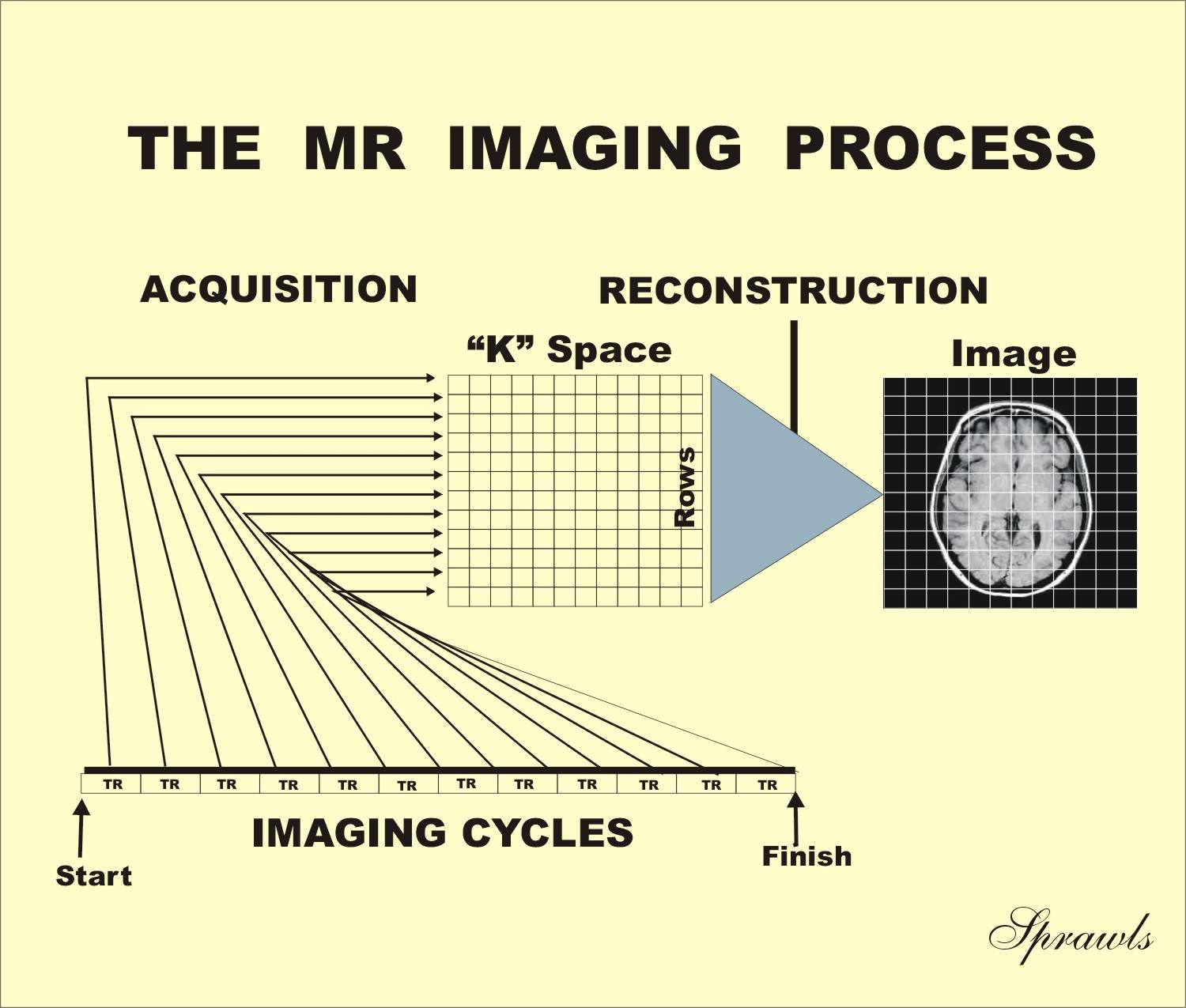 |
In this chapter we will develop a general overview of the imaging process
and set the stage for considering the different methods and techniques that are
used to produce optimum images for various clinical needs
The
image reconstruction process is usually fast compared to the acquisition process
and generally does not require any decisions or adjustments by the operator.
Each
imaging procedure is controlled by a protocol that has been entered into the
computer. Issues that must be considered in selecting, modifying, or developing
a protocol for a specific clinical procedure include:
In the following chapters we will address each of these issues and the
specific protocol factors that are used to produce the desired image
characteristics.
|
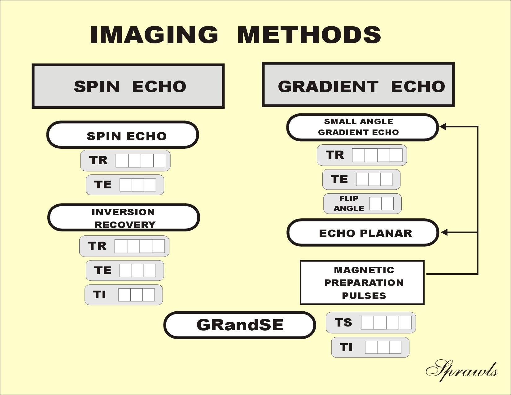
Figure 5-2. The principal spin echo and gradient
echo imaging methods. GRandSE, or GRASE, is a combination of the two
methods. |
 |
The selection of a specific imaging method and factor values is generally
based on requirements for contrast sensitivity to a specific tissue
characteristic (PD, T1, T2) and acquisition speed. However, other
characteristics such as visual noise and the sensitivity to specific artifacts
might vary from method to method.
All of the imaging methods belong to one or both of the two major
families, spin echo or gradient echo. The difference between the
two families of methods is the process that is used to create the echo event at
the end of each imaging cycle. For the spin echo methods, the echo event is
produced by the application of a 180° RF pulse, as will be described in Chapter
6. For the gradient echo methods the event is produced by applying a magnetic
field gradient, as described in Chapter 7. Each method has very specific
characteristics and applications.
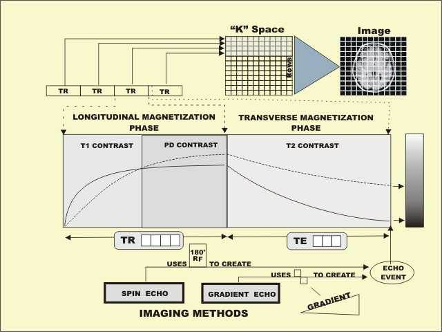
A common characteristic of all methods is that there are two distinct phases of the image acquisition cycle, as shown in Figure 5-3.
|
Figure 5-3. The longitudinal and transverse
magnetization phases of an imaging cycle. T1 and PD contrast are
produced during the longitudinal phase and T2 contrast is produced
during the transverse phase. |
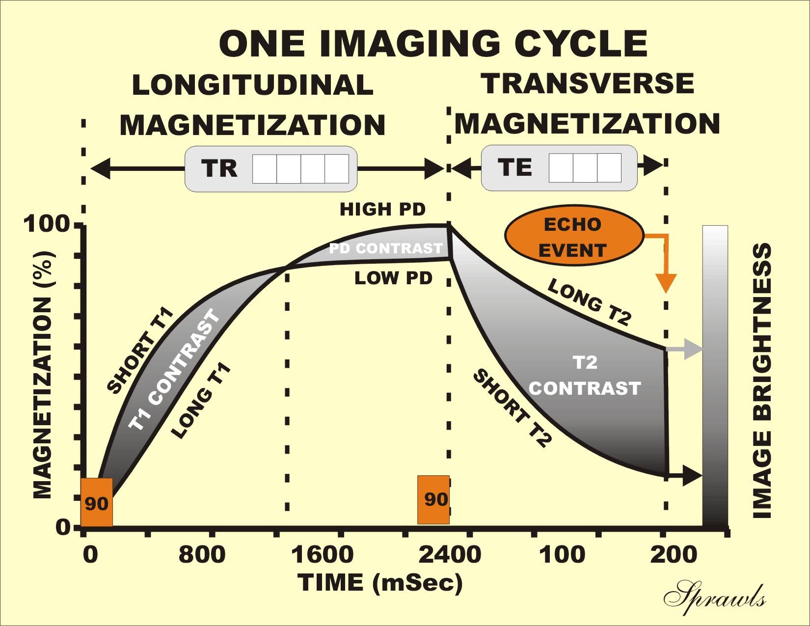 |
One
phase is associated with longitudinal magnetization and the other with
transverse magnetization. In general, T1 contrast is developed during the
longitudinal magnetization phase and T2 contrast is developed during the
transverse magnetization phase. PD contrast is always present, but becomes most
visible when it is not overshadowed by either T1 or T2 contrast. The predominant
type of contrast that ultimately appears in the image is determined by the
duration of the two phases and the transfer of contrast from the longitudinal
phase to the transverse phase.
The duration of the two phases (longitudinal and transverse) is
determined by the selected values of the protocol factors, TR (Time of
Repetition) and TE (Time to Echo).
TR is
the time interval between the beginning of the longitudinal relaxation,
following saturation, and the time at which the longitudinal magnetization is
converted to transverse magnetization by the excitation pulse. This is when the
picture is snapped relative to the longitudinal magnetization.
Because the longitudinal relaxation takes a relatively long time, TR is
also the duration of the image acquisition cycle or the cycle repetition time
(Time of Repetition).
The
excitation pulse is characterized by a flip angle. A 90˚ excitation pulse
converts all of the existing longitudinal magnetization into transverse
magnetization. This type of pulse is used in the spin echo methods. However,
there are methods that use excitation pulses with flip angles that are less than
90˚. Small flip angles (<90˚) convert only a fraction of the existing
longitudinal magnetization into transverse magnetization and are used primarily
to reduce acquisition time with the gradient echo methods described in Chapter
7.
The
transverse magnetization phase terminates with the echo event, which produces
the RF signal. This is the signal that is emitted by the tissue and used to form
the image. The echo event is produced by applying either an RF pulse or a
gradient pulse to the tissue, as will be described in Chapters 6 and 7
During the relaxation (regrowth) of longitudinal magnetization, different tissues will have different levels of magnetization because of their different growth rates, or T1 values. Figure 5-4 compares two tissues with different T1 values.
|
Figure 5-4. The amount of T1 contrast captured
during the longitudinal magnetization phase is determined by the value
of TR that is selected by the operator. |
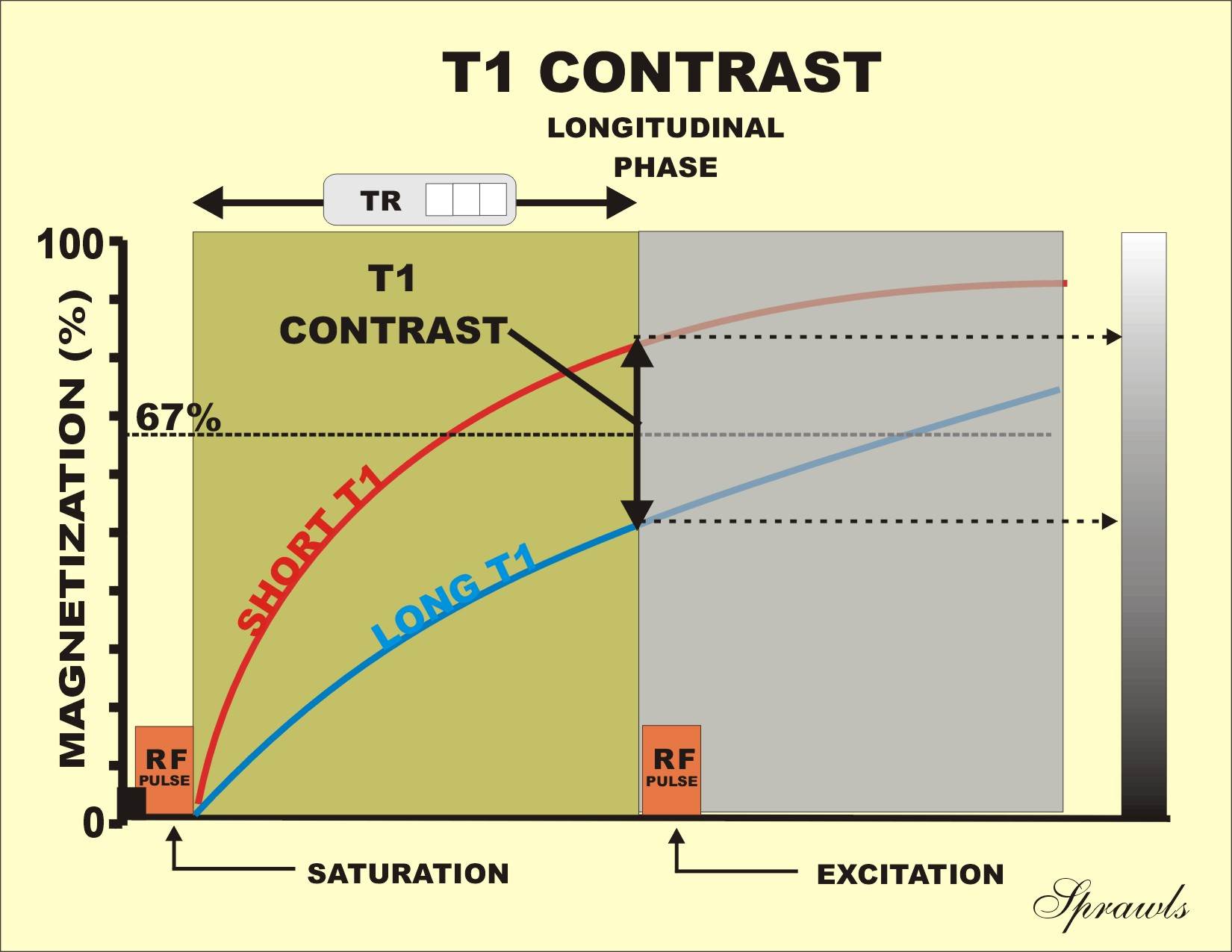 |
The tissue with the shorter T1 value experiences a faster regrowth of
longitudinal magnetization. Therefore, during this period of time it will have a
higher level of magnetization, produce a more intense signal, and appear
brighter in the image. In T1-weighted images brightness or high signal intensity
is associated with short T1 values.
t the beginning of each imaging cycle, the longitudinal magnetization is
reduced to zero (saturation) by an RF pulse, and then allowed to regrow, or
relax. This is what happens in the spin echo method. In some other imaging
methods, as we will see in the next two chapters, the cycle might begin with
either partially saturated or inverted longitudinal magnetization. In all cases,
T1 contrast is formed during the regrowth process. At a time determined by the
selected TR value, the cycle is terminated and the magnetization value is
converted to transverse, measured and displayed as a pixel intensity, or
brightness, and a T1-weighted image is produced.
In principle, at the beginning of each imaging cycle all tissues are
dark. As the tissues regain longitudinal magnetization, they become brighter.
The brightness, or intensity, with which they appear in the image depends on
when during the regrowth process the cycle is terminated and the picture is
snapped. This is determined by the selected TR value. When a short TR is used,
the regrowth of the longitudinal magnetization is interrupted before it reaches
its maximum. This reduces signal intensity and tissue brightness within the
image but produces T1 contrast.
Increasing TR increases signal intensity and brightness up to the point
at which magnetization is fully recovered, which is determined by the PD of each
tissue. For practical purposes, this occurs when the TR exceeds approximately
three times the T1 value for the specific tissues. Although it takes many cycles
to form a complete image, the longitudinal magnetization is always measured at
the same time in each cycle as determined by the setting of TR.
To produce a T1-weighted image, a value for TR must be selected to
correspond with the time at which T1 contrast is significant between the two
tissues. Several factors must be considered in selecting TR. If T1 contrast is
represented by the ratio of the tissue magnetization levels, it is at its
maximum very early in the relaxation process. However, the low magnetization
levels present at that time do not generally produce adequate RF signal levels
for many clinical applications. The selection of a longer TR produces greater
signal strength but less T1 contrast.
The selection of TR must be appropriate for the T1 values of the tissues
being imaged. If a TR value is selected that is equal to the T1 value of a
tissue, the picture will be snapped when the tissue has regained 63% of its
magnetization. This represents the time when there is maximum contrast between
tissues with small differences in T1 values.
|
Figure 5-5. Proton density
(PD) contrast is captured by setting TR to relatively long values. At
that time the magnetization is determined by PD and is not T1 as in the
earlier part of the cycle. |
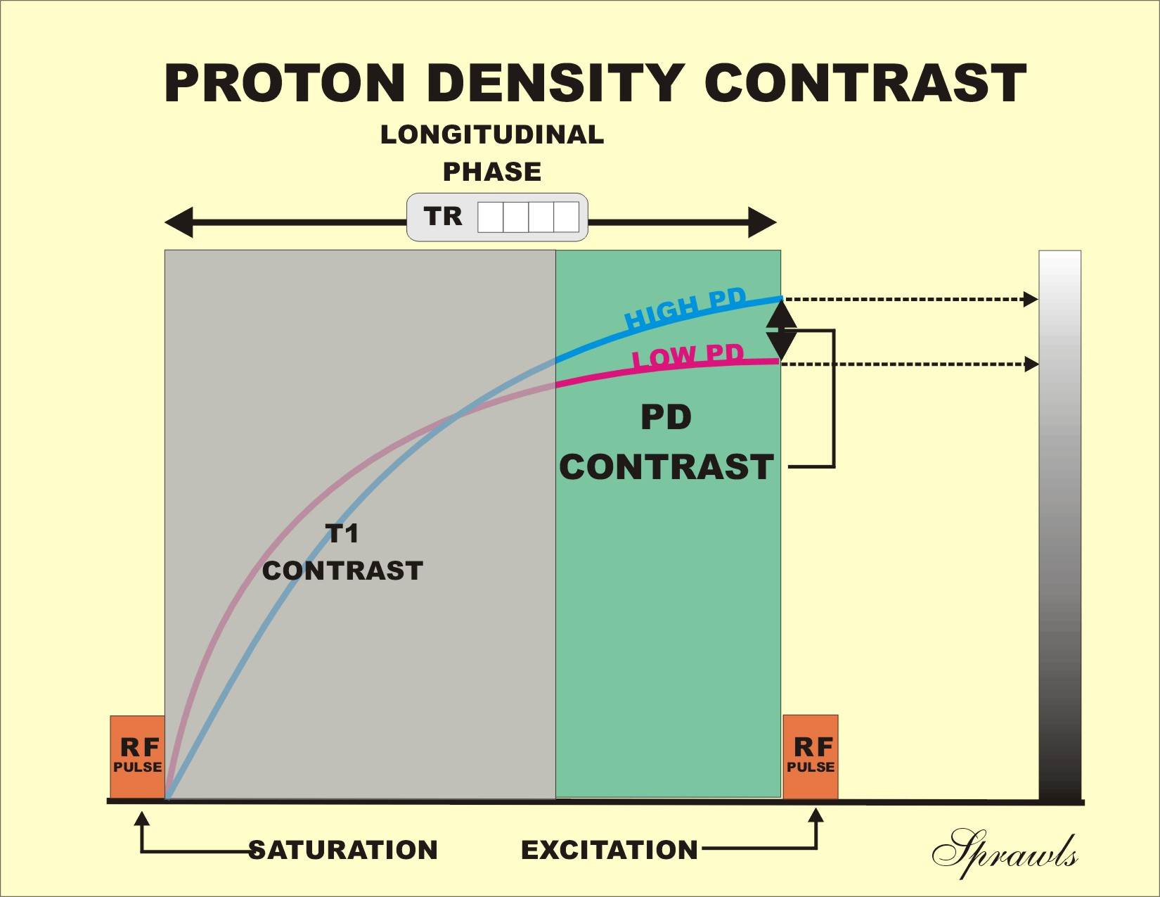 |
Here
we see the growth of longitudinal magnetization for two tissues with the same T1
values but different relative PDs. The tissue with the lowest PD (80) reaches a
maximum magnetization level that is only 80% that of the other tissue. The
difference in magnetization levels at any point in time is because of the
difference in PD and is therefore the source of PD contrast.
Although there is some PD contrast early in the cycle, it is generally
quite small in comparison to the T1 contrast.
The basic difference between T1 contrast and PD contrast is that T1
contrast is produced by the rate of growth (relaxation), and PD contrast is
produced by the maximum level to which the magnetization grows. In general, T1
contrast predominates in the early part of the relaxation phase, and PD contrast
predominates in the later portion. T1 contrast gradually gives way to PD
contrast as magnetization approaches the maximum value. A PD-weighted image is
produced by selecting a relatively long TR value so that the image is created or
“the picture is snapped” in the later portion of the relaxation phase, where
tissue magnetizations approach their maximum values. The TR values at which this
occurs depend on the T1 values of the tissues being imaged.
It was shown earlier that tissue reaches 95% of its magnetization in
three T1s. Therefore, a TR value that is at least three times the T1 values for
the tissues being imaged produces almost pure PD contrast.
Now let
us turn our attention to the transverse phase. During the decay of transverse
magnetization, different tissues will have different levels of magnetization
because of different decay rates, or T2 values. As shown in Figure 56, tissue
with a relatively long T2 value will have a higher level of magnetization,
produce a more intense signal, and appear brighter in the image than a tissue
with a shorter T2 value.
Figure 5-6 shows the decay of transverse magnetization for tissues with
different T2 values. The tissue with the shortest T2 value loses its
magnetization faster than the other tissues.
|
Figure 5-6. The formation of T2 contrast during
the transverse magnetization phase. The amount of T2 contrast captured
depends on the selected value of TE, the Time to Echo event. |
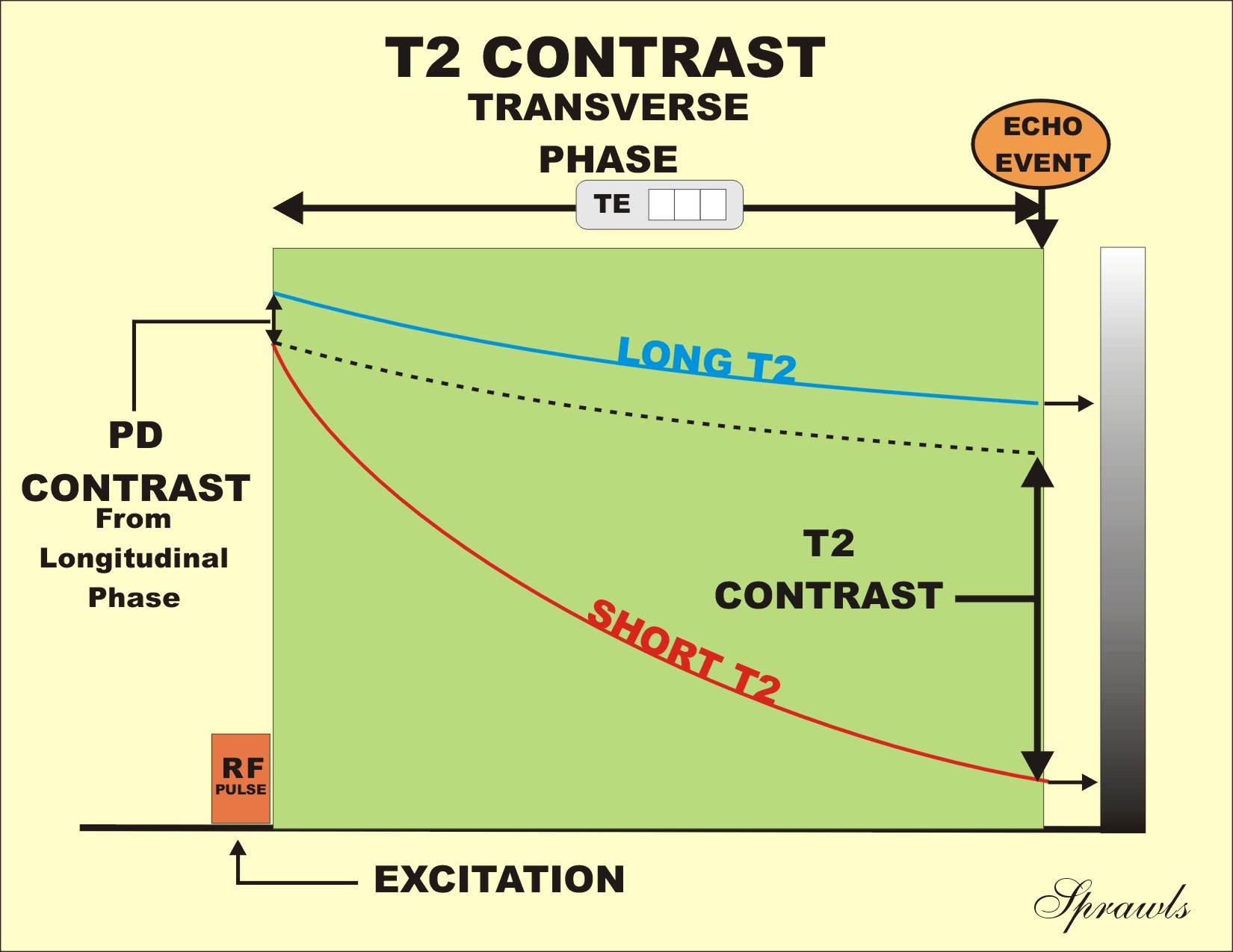 |
The difference in T2 values of tissue can be translated into image
contrast. For the purpose of this illustration we assume that the two tissues
begin their transverse relaxation with the levels of magnetization determined by
the PD. This is the usual case where the PD contrast present at the end of the
longitudinal phase carries over to the beginning of the transverse phase. In
effect, the transverse phase begins with PD contrast but adds T2 contrast as
time elapses. The decay of the magnetization proceeds at different rates because
of the different T2 values. The tissue with the longer T2 value maintains a
higher level of magnetization than the other tissue and will remain bright
longer. The difference in the tissue magnetizations at any point in time
represents contrast.
At the beginning of the cycle there is no T2 contrast, but it develops
and increases throughout the relaxation process. At the echo event the
magnetization levels are converted into RF signals that are displayed as image
pixel brightness; this is the time to echo event (TE) and is selected by the
operator. Maximum T2 contrast is generally obtained by using a relatively long
TE. However, when a very long TE value is used, the magnetization and the RF
signals might be too low to form a useful image. In selecting TE values, a
compromise must often be made between T2 contrast and good signal intensity.
The transverse magnetization characteristics of tissue (T2 values) are,
in principle, added to the longitudinal characteristics carried over from the
longitudinal phase (e.g., T1 and PD) to form the MR image. Usually we do not
want to add T2 contrast to T1 contrast. That is because these two types of
contrast oppose each other. Remember in Chapter 1 we saw that tissues that are
bright in T1 images are dark in T2 images. This means that if we were to mix T1
and T2 contrast in the same image, one would cancel the other. When setting up a
protocol for a T2 image it is necessary to use a long TR (in addition to a long
TE) so that no, or very little, T1 contrast carries over to the transverse
phase.
The Imaging Process
After application of a saturation pulse, which reduces the longitudinal
magnetization to zero, the magnetization begins to regrow, a process known as
relaxation. The rate of regrowth for a specific tissue is determined by that
tissue’s T1 value. Tissues with short T1 values grow faster than tissues with
long T1 values. During this regrowth, T1 contrast in the form of different
levels of magnetization is created among the tissues. This is the contrast that
will be displayed in an image if the protocol parameters are set to produce a
T1-weighted image. In a T1-weighted image, tissues with short T1 values will be
bright. Tissues and fluid with long T1 values will be darker.
When an RF pulse is applied to longitudinal magnetization, it converts
(flips) it to transverse magnetization, an unstable excited magnetic condition
that decays with time. This decay process is the transverse magnetization
relaxation process. The rate of decay of a specific tissue depends on that
tissue’s T2 value. Tissues with short T2 values decay faster than tissues with
longer T2 values. When the imaging protocol factors are set to produce a
T2-weighted image, tissues with short T2 values will be dark and tissues and
fluids with longer T2 values will be bright.